Beginner’s Guide For Data Analysis Using SQL
This article was published as a part of the Data Science Blogathon
Overview
This article provides an overview of data analysis using SQL, which should be a must-have tool for any data scientist – both for gaining access to data and, more importantly, as a basic tool for advanced data analysis. The idea behind SQL is fairly similar to any other tool or language used for data analysis (excel, Pandas), and should be very intuitive to people who have worked with data before.
Important Definitions
SQL is a programming language that allows you to work with data stored in databases. SQLite is the specific implementation in this scenario. All of the capabilities listed in this document are available in most SQL languages. Performance and advanced analytical functions are usually the areas where there are variances (and sometimes bugs of course). We’ll eventually use SQL to build queries that get data from the database, manipulate it, sort it, and extract it.
The most significant part of the database is its tables, which contain all of the data. Normally, data would be divided among several tables rather than being saved all in one location (so designing the data structure properly is very important). The majority of this script would deal with table manipulation. Aside from tables, there are a few more extremely helpful concepts/features that we will not discuss:
- table creation
- inserting/updating data in the database
- functions – takes a value as an input and returns a value that has been manipulated (for example function that remove white spaces)
#Improts

import numpy as np # linear algebra

import pandas as pd # data processing, CSV file I/O (e.g. pd.read_csv)

import sqlite3

import matplotlib.pyplot as plt

# Load data from database.sqlite

database = 'database.sqlite'
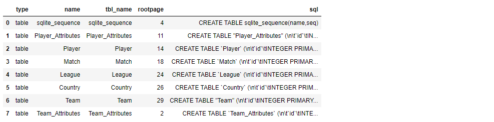
We’ll start by connecting to the database and seeing what tables we have.
The query’s basic structure is straightforward: After the SELECT, you specify what you wish to see; * denotes all possible columns. Following the FROM, you select the table. After the WHERE, you add the conditions for the data you wish to use from the table(s).
The section’s structure and order of content, with spaces, new lines, capital letters, and indentation to make the code easier to understand.
conn = sqlite3.connect(database)
tables = pd.read_sql("""SELECT *
                        FROM sqlite_master
                        WHERE type='table';""", conn)
tables
List of countries
This is the most basic query. The only must part of a query is the SELECT and the FROM (assuming you want to pull from a table)
countries = pd.read_sql("""SELECT *
                        FROM Country;""", conn)
countries

List of leagues and their country
When you wish to link two tables together, you use JOIN. When you have a common key in each of them, it works. Understanding the concept of keys is essential for linking (joining) data sets (tables). Each entry (row) in a table is uniquely identified by a key. It might be made up of a single value (cell) – commonly ID – or a group of values that are all unique in the table.
When joining tables, you must do the following:
INNER JOIN – only maintain records in both tables that match the criterion (after the ON), and records from both tables that don’t match won’t appear in the output.
LEFT JOIN – all values from the first (left) table are combined with the matching rows from the right table. NULL values would be assigned to the columns from the right table that doesn’t have a corresponding value in the left table.
Specify the common value that will be used to link the tables together (the id of the country in that case).
Ensure that at least one of the values in the table is a key. It’s the Country.id in our case. Because there can be more than one league in the same nation, the League.country id is not unique.
Using JOINS incorrectly is the most common and dangerous mistake when writing complex queries.
leagues = pd.read_sql("""SELECT *
                        FROM League
                        JOIN Country ON Country.id = League.country_id;""", conn)
leagues

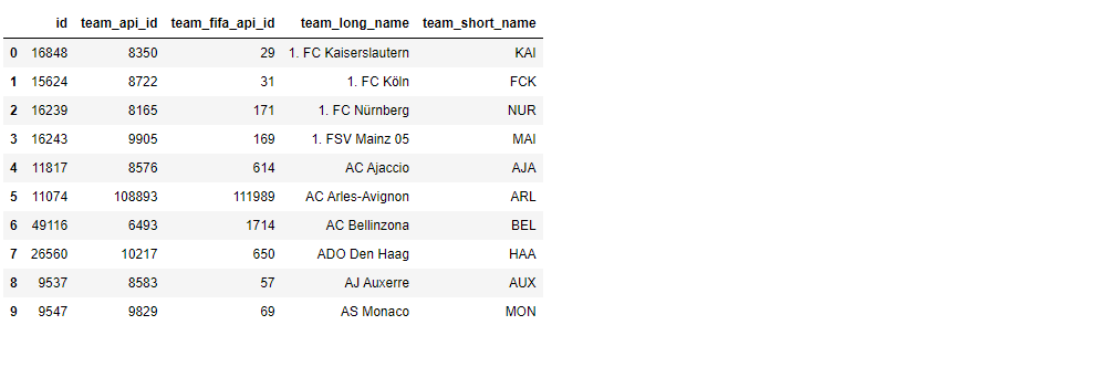
List of teams
ORDER BY defines the sorting of the output – ascending or descending (DESC)
LIMIT limits the number of rows in the output – after the sorting
teams = pd.read_sql("""SELECT *
                        FROM Team
                        ORDER BY team_long_name
                        LIMIT 10;""", conn)
teams
We’ll just show the columns that interest us in this example, so instead of *, we’ll use the actual names.
The names of several of the cells are the same (Country.name, League.name). We’ll use AS to rename them.
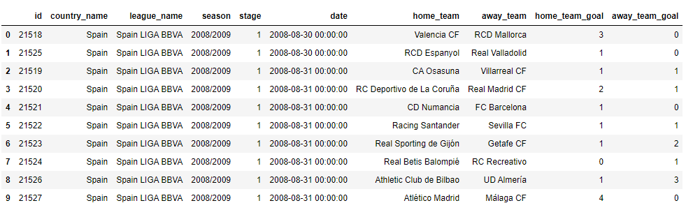
This query, as you can see, includes a lot more joins. The reason for this is that the database is designed in a star structure, with one table (Match) containing all of the “performance” and metrics, but only keys and IDs, and other tables including all of the descriptive information (Country, League, Team)
It’s important to note that the Team is joined twice. This is a hard one because, despite the fact that we are using the same table name, we are bringing two separate copies (and rename them using AS). The reason for this is that we need to bring data for two separate values (home team API id and away team API id), and joining them to the same database would imply that they are equal.
It’s also worth noting that the Team tables are linked together using a left join. The reason for this is that I’ve decided to keep the matches in the output, even if one of the teams isn’t on the Team table.
ORDER comes before LIMIT and after WHERE and determines the output order.
detailed_matches = pd.read_sql("""SELECT Match.id,
                                        Country.name AS country_name,
                                        League.name AS league_name,
                                        season,
                                        stage,
                                        date,
                                        HT.team_long_name AS  home_team,
                                        AT.team_long_name AS away_team,
                                        home_team_goal,
                                        away_team_goal
                                FROM Match
                                JOIN Country on Country.id = Match.country_id
                                JOIN League on League.id = Match.league_id
                                LEFT JOIN Team AS HT on HT.team_api_id = Match.home_team_api_id
                                LEFT JOIN Team AS AT on AT.team_api_id = Match.away_team_api_id
                                WHERE country_name = 'Spain'
                                ORDER by date
                                LIMIT 10;""", conn)
detailed_matches
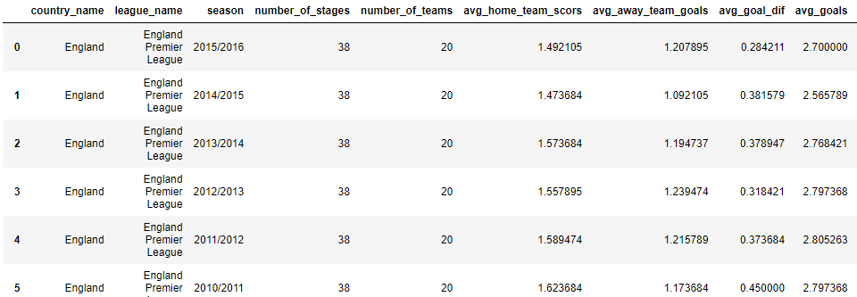
Let’s do some basic analytics
The functionality we will use for that is GROUP BY, which comes between the WHERE and ORDER
Once you chose what level you want to analyze, we can decide the select statement into two:
Dimensions are the values we’re describing, and they’re the same ones we’ll group by later.
Metrics must be grouped together using functions. sum(), count(), count(distinct), avg(), min(), and max() are some of the most common functions.
It’s critical to use the same dimensions in both the select and the GROUP BY functions. Otherwise, the output could be incorrect.
HAVING is another feature that can be used after grouping. This adds another layer of data filtering, this time using the table’s output after grouping. It’s frequently used to clean the output.
leages_by_season = pd.read_sql("""SELECT Country.name AS country_name,
                                        League.name AS league_name,
                                        season,
                                        count(distinct stage) AS number_of_stages,
                                        count(distinct HT.team_long_name) AS number_of_teams,
                                        avg(home_team_goal) AS avg_home_team_scors,
                                        avg(away_team_goal) AS avg_away_team_goals,
                                        avg(home_team_goal-away_team_goal) AS avg_goal_dif,
                                        avg(home_team_goal+away_team_goal) AS avg_goals,
                                        sum(home_team_goal+away_team_goal) AS total_goals
                                FROM Match
                                JOIN Country on Country.id = Match.country_id
                                JOIN League on League.id = Match.league_id
                                LEFT JOIN Team AS HT on HT.team_api_id = Match.home_team_api_id
                                LEFT JOIN Team AS AT on AT.team_api_id = Match.away_team_api_id
                                WHERE country_name in ('Spain', 'Germany', 'France', 'Italy', 'England')
                                GROUP BY Country.name, League.name, season
                                HAVING count(distinct stage) > 10
                                ORDER BY Country.name, League.name, season DESC
                                ;""", conn)
leages_by_season
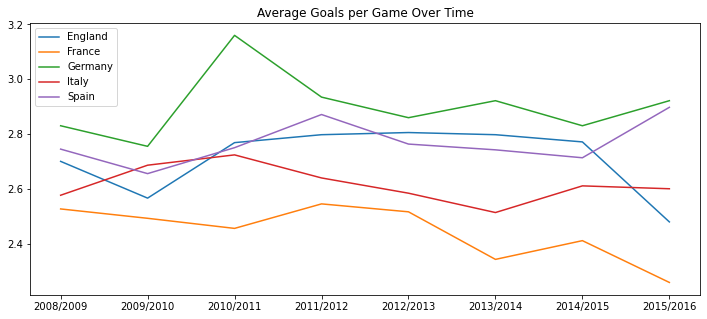
df = pd.DataFrame(index=np.sort(leages_by_season['season'].unique()), columns=leages_by_season['country_name'].unique())
df.loc[:,'Germany'] = list(leages_by_season.loc[leages_by_season['country_name']=='Germany','avg_goals'])
df.loc[:,'Spain']   = list(leages_by_season.loc[leages_by_season['country_name']=='Spain','avg_goals'])
df.loc[:,'France']   = list(leages_by_season.loc[leages_by_season['country_name']=='France','avg_goals'])
df.loc[:,'Italy']   = list(leages_by_season.loc[leages_by_season['country_name']=='Italy','avg_goals'])
df.loc[:,'England']   = list(leages_by_season.loc[leages_by_season['country_name']=='England','avg_goals'])
df.plot(figsize=(12,5),title='Average Goals per Game Over Time')
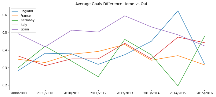
df = pd.DataFrame(index=np.sort(leages_by_season['season'].unique()), columns=leages_by_season['country_name'].unique())
df.loc[:,'Germany'] = list(leages_by_season.loc[leages_by_season['country_name']=='Germany','avg_goal_dif'])
df.loc[:,'Spain']   = list(leages_by_season.loc[leages_by_season['country_name']=='Spain','avg_goal_dif'])
df.loc[:,'France']   = list(leages_by_season.loc[leages_by_season['country_name']=='France','avg_goal_dif'])
df.loc[:,'Italy']   = list(leages_by_season.loc[leages_by_season['country_name']=='Italy','avg_goal_dif'])
df.loc[:,'England']   = list(leages_by_season.loc[leages_by_season['country_name']=='England','avg_goal_dif'])
df.plot(figsize=(12,5),title='Average Goals Difference Home vs Out')
Query Run Order
Now that we are familiar with most of the functionalities being used in a query, it is very important to understand the order that code runs.
First, order of how we write it (reminder):
- SELECT
- FROM
- JOIN
- WHERE
- GROUP BY
- HAVING
- ORDER BY
- LIMIT
Now, let’s look at the actual sequence of events. To begin, consider this section as constructing a new temporal table in your memory:
- Define which tables will be used and how they will be connected (FROM + JOIN).
- Only the rows that apply to the conditions should be kept (WHERE)
- Sort the information by the required level (if need) (BY GROUP)
- Select the data you wish to include in the new table. It can contain only raw data (if there is no grouping), or a combination of dimensions (from the grouping), as well as metrics. You’ve decided to show the following from the table.
- Order the new table’s output (ORDER BY)
- Add extra filtering conditions to the newly generated table (HAVING)
- Limit the number of rows – this would reduce the number of rows, as well as the need for filtering (LIMIT)
Sub Queries and Functions
Using subqueries is an essential tool in SQL, as it allows manipulating the data in very advanced ways without the need of any external scripts, and especially important when your tables are structured in such a way that you can’t be joined directly.
In our example, we attempting to connect a table that contains basic player information (name, height, and weight) to a table that contains additional qualities. The difficulty is that, while the first table has one row for each player, the second table’s key is player+season, thus a typical join would result in a Cartesian product, with each player’s basic data appearing as many times as this player appears in the attributes table. Of course, this has the drawback of skewing the average in favor of players who feature frequently in the attribute table.
Use a subquery as a solution. The attributes database would need to be grouped to a different key-player level only (without season). Of course, we would need to decide first how we would want to combine all the attributes to a single row. use AVG, also one can decide on maximum, latest season and etc. Once both tables have the same keys, we can join them together (think of the subquery like any other table, only temporal), knowing that we won’t have duplicated rows after the join.
You can also see two examples of how to use functions here:
– A conditional function is an important tool for data manipulation. While the IF statement is widely used in other languages, SQLite does not support it, hence CASE + WHEN + ELSE is used instead. As you can see, the query would return varied results depending on the data input.
– ROUND – straightforward. Every SQL language comes with a lot of useful functions by default.
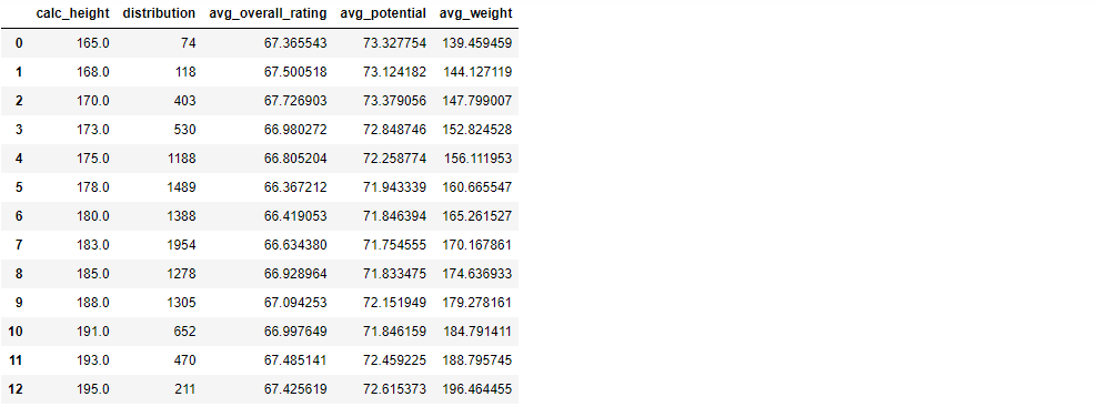
players_height = pd.read_sql("""SELECT CASE
                                        WHEN ROUND(height)<165 then 165
                                        WHEN ROUND(height)>195 then 195
                                        ELSE ROUND(height)
                                        END AS calc_height,
                                        COUNT(height) AS distribution,
                                        (avg(PA_Grouped.avg_overall_rating)) AS avg_overall_rating,
                                        (avg(PA_Grouped.avg_potential)) AS avg_potential,
                                        AVG(weight) AS avg_weight
                            FROM PLAYER
                            LEFT JOIN (SELECT Player_Attributes.player_api_id,
                                        avg(Player_Attributes.overall_rating) AS avg_overall_rating,
                                        avg(Player_Attributes.potential) AS avg_potential
                                        FROM Player_Attributes
                                        GROUP BY Player_Attributes.player_api_id)
                                        AS PA_Grouped ON PLAYER.player_api_id = PA_Grouped.player_api_id
                            GROUP BY calc_height
                            ORDER BY calc_height
                                ;""", conn)
players_height
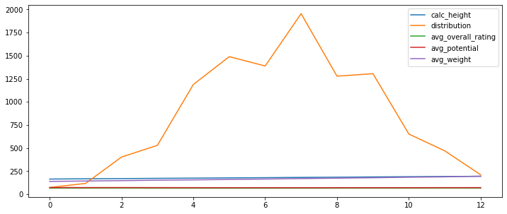
players_height.plot(figsize=(12,5))
So, SQL is a programming language that allows you to work with data stored in databases, and also we can analyze row data from databases.
EndNote
Thank you for reading!
I hope you enjoyed the article and increased your knowledge.
Please feel free to contact me on Email
Something not mentioned or want to share your thoughts? Feel free to comment below And I’ll get back to you.
About the Author
Hardikkumar M. Dhaduk
Data Analyst | Digital Data Analysis Specialist | Data Science Learner
Connect with me on Linkedin
Connect with me on Github


