Machine learning is an amazing tool for many tasks. OpenCV is a great library for manipulating images. It would be great if we can put them together.
In this 7-part crash course, you will learn from examples how to make use of machine learning and the image processing API from OpenCV to accomplish some goals. This mini-course is intended for practitioners who are already comfortable with programming in Python, know the basic concept of machine learning, and have some background in manipulating images. Let’s get started.
Machine Learning in OpenCV (7-day Mini-Course) Photo by Nomadic Julien. Some rights reserved.
Who Is This Mini-Course For?
Before we get started, let’s make sure you are in the right place. The list below provides some general guidelines as to who this course was designed for. Don’t panic if you don’t match these points exactly, you might just need to brush up in one area or another to keep up.
Developers that know how to write a little code. This means that it is not a big deal for you to get things done with Python and know how to setup the ecosystem on your workstation (a prerequisite). It does not mean you’re a wizard coder, but it does mean you’re not afraid to install packages and write scripts.
Developers that know a little machine learning. This means you know about some common machine learning algorithms like regression or neural networks. It does not mean that you are a machine learning PhD, just that you know the landmarks or know where to look them up.
Developers that know a bit about image processing. This means you know how to read an image file, how to manipulate a pixel, and how to crop a sub-image. Preferably using OpenCV. It does not mean that you are an image processing expert but you understand that digital images are arrays of pixels.
This mini-course is not a textbook on machine learning, OpenCV, or digital image processing. Rather, it is a project guideline that takes you step-by-step from a developer with minimal knowledge to a developer who can confidently use machine learning in OpenCV.
Mini-Course Overview
This mini-course is divided into 7 parts.
Each lesson was designed to take the average developer about 30 minutes. You might finish some much sooner and other you may choose to go deeper and spend more time.
You can complete each part as quickly or as slowly as you like. A comfortable schedule may be to complete one lesson per day over seven days. Highly recommended.
The topics you will cover over the next 7 lessons are as follows:
Lesson 1: Introduction to OpenCV
Lesson 2: Read and Display Images Using OpenCV
Lesson 3: Finding Circles
Lesson 4: Extracting Subimages
Lesson 5: Matching Pennies
Lesson 6: Building a Coin Classifier
Lesson 7: Using DNN Module in OpenCV
This is going to be a lot of fun.
You’re going to have to do some work though, a little reading, a little research and a little programming. You want to learn machine learning and computer vision right?
Post your results in the comments; I’ll cheer you on!
Hang in there; don’t give up.
Lesson 01: Introduction to OpenCV
OpenCV is a popular open source library for processing images. It has API bindings in Python, C++, Java, and Matlab. It comes with thousands of functions and implemented many advanced image processing algorithms. If you’re using Python, a common alternative to OpenCV is PIL (Python Imaging Library, or its successor, Pillow). Compared to PIL, OpenCV has a richer set of features and is often faster because it is implemented in C++.
This mini-course is to apply machine learning in OpenCV. In later lessons of this mini-course, you will also need TensorFlow/Keras and tf2onnx library in Python.
In this lesson your goal is to install OpenCV.
For a basic Python environment, you can install packages using pip. To install OpenCV using pip, together with TensorFlow and tf2onnx, you can use:
1
sudo pip install opencv-python tensorflow tf2onnx
OpenCV is named as package opencv-python in PyPI, but it contains only the “free” algorithms and main modules. There is also the package opencv-contrib-python, which also included the “extra” modules. These extra modules are less stable and not well-tested. If you prefer to install the latter, you should use the following commmand instead:
However, if you’re using Anaconda or miniconda environment, the name of the package is just opencv, which you can install with the command conda install.
To know your OpenCV installation works, you can simply run a simple script and check its version:
Repeat the above code to make sure you have OpenCV correctly installed. Can you also print the version of TensorFlow module by adding a few lines to the code?
In the next lesson, you will use OpenCV to read and display an image.
Lesson 02: Read and Display Image Using OpenCV
OpenCV, the Open Source Computer Vision Library, is a powerful tool for image processing and computer vision tasks. But before diving into complex algorithms, let’s master the basics: reading and displaying images.
Reading an image using OpenCV is to use cv2.imread() function. It takes the path to the image file and returns a NumPy array. The array would usually be three-dimensional, in height×width×channel and each element is an unsigned 8-bit integer. “Channel” is usually BGR (blue-green-red) in OpenCV. But if you prefer to load the image in grayscale, you can add an extra parameter, such as:
The code above will print the array dimension. While we usually describe an image as width×height, array dimension is described as height×width. If the image is read in grayscale, there is only one channel and hence the output will be a two-dimensional array.
If you removed the second argument to make it simply cv2.imread("path/filename.jpg"), the array should be in shape height×width×3 for three channels of BGR.
To display an image, you can use OpenCV’s cv2.imshow() function. This will create a window to display the image. But this window will not be shown unless you ask OpenCV to wait for you to interact with the window. Normally, you use:
1
2
3
4
...
cv2.imshow("My image",image)
cv2.waitKey(0)
cv2.destroyAllWindows()
The cv2.imshow() takes the window title as its first argument. The image to display should be in BGR channel order. The cv2.waitKey() function will wait for your key press for certain milliseconds as specified in its function argument. If zero, it will wait indefinitely. The key press will be returned as its codepoint in integer, which in this case, you ignored it. As a good practice, you closed the window before this program ends.
Modify the code above to point the path to an image in your disk and try it out. How can you modify the code above to wait until Esc key is pressed but ignoring all other keys? (Hint: The code point for Esc key is 27)
In the next lesson, you will see how to find patterns in an image.
Lesson 03: Finding Circles
Since a digital image is represented as a matrix, you can devise your algorithm and check each pixel of the image to identify if some pattern exists in the image. Over the years, a lot of clever algorithms have been invented and you can learn some of them in any digital image processing textbook.
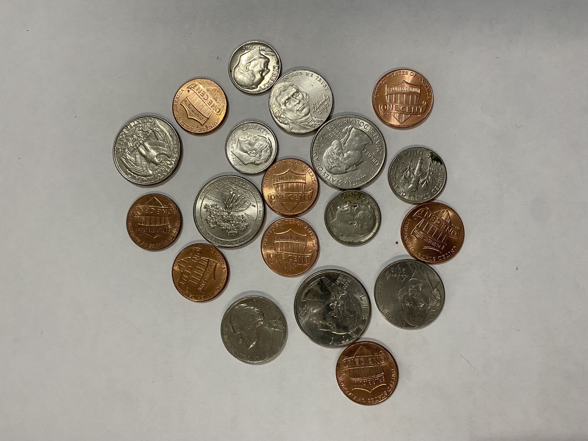
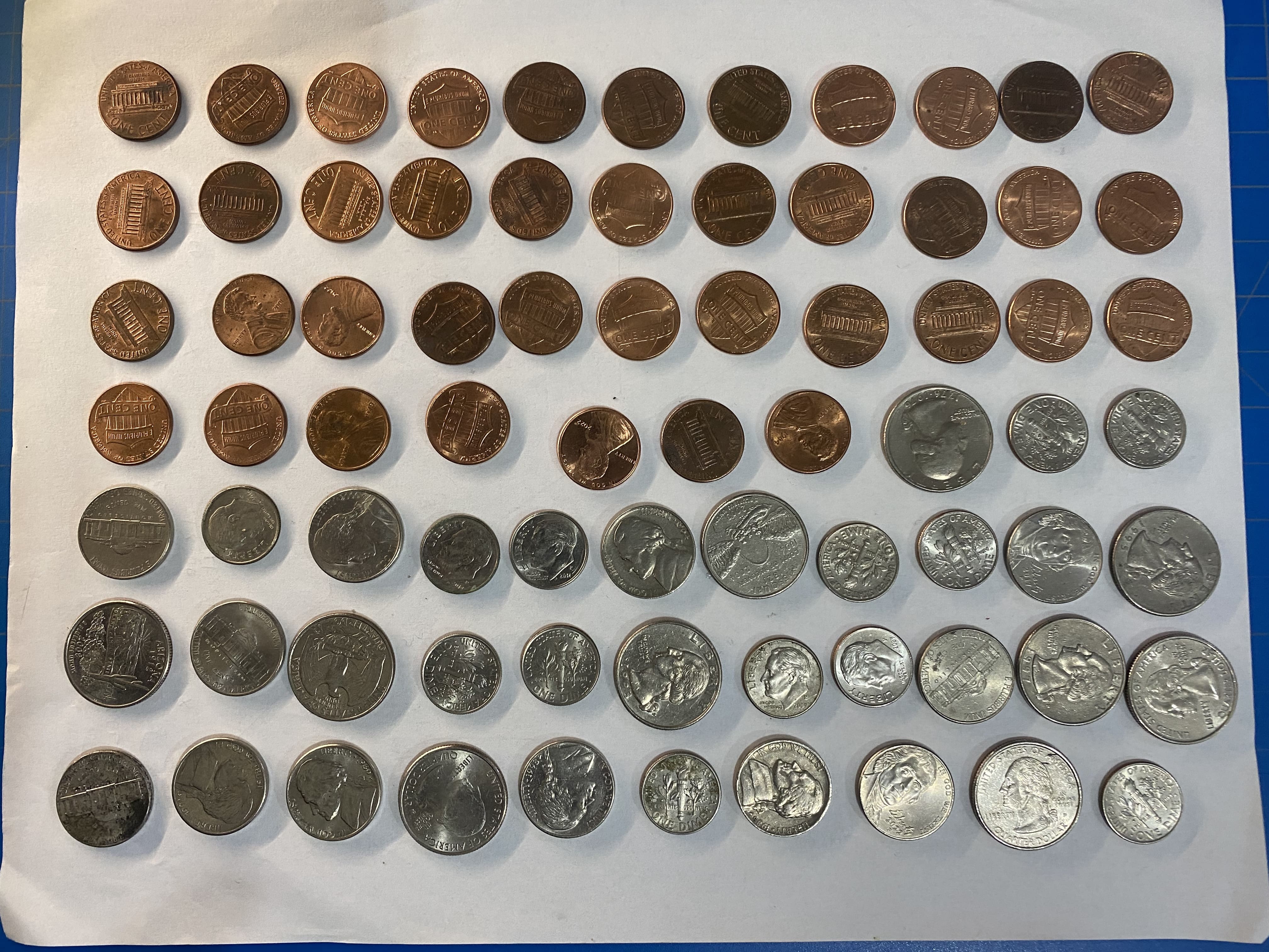
In this mini-course, you’re going to solve a simple problem: Given an image with many coins, identify and count a particular type of coin. Coins are circles. To identify circles in an image, one promising algorithm is to use the Hough Circle Transform.
Hough Transform is an algorithm that makes use of gradient information of an image. Therefore, it works on a grayscale image rather than a color image. To convert a colored image to grayscale, you can use the cv2.cvtColor() function from OpenCV. Because Hough Transform is based on gradient information, it would be sensitive to image noise. Applying Gaussian blur is a usual preprocessing step to reduce noise for Hough Transform. In code, you apply the following for a BGR image you read:
1
2
3
...
gray=cv2.cvtColor(img,cv2.COLOR_BGR2GRAY)
blur=cv2.GaussianBlur(gray,(25,25),1)
Here the Gaussian blur is applied using a $25\times 25$ kernel. You can use a smaller or larger kernel depending on the level of noise in the image.
Hough Circle Transform is to find circles from an image, using the following function:
There are a lot of parameters. The first argument is the grayscale image and the second is the algorithm to use. The rest are as follows:
dp: Ratio of image resolution to accumulator resolution. Use 1.0 to 2.0 normally.
minDist: Minimum distance between centers of detected circles. The lesser the value, the more false positives you will get.
param1 This is the threshold for the Canny edge detector
param2: When algorithm cv2.HOUGH_GRADIENT is used, this is the accumulator threshold. The lesser the value, the more false positives.
minRadius and maxRadius: Minimum and maximum circle radius to detect
The returned value from the function cv2.HoughCircles() is a NumPy array of circles, represented as rows containing the center coordinates and the radius.
Download the image, save it as coins-1.jpg, and run the following code:
1
2
3
4
5
6
7
8
9
10
11
12
13
14
15
16
17
import cv2
import numpy asnp
image_path="coins-1.jpg"
img=cv2.imread(image_path)
gray=cv2.cvtColor(img,cv2.COLOR_BGR2GRAY)
blur=cv2.GaussianBlur(gray,(25,25),1)
circles=cv2.HoughCircles(blur,cv2.HOUGH_GRADIENT,
dp=1,minDist=100,
param1=80,param2=60,minRadius=90,maxRadius=150)
ifcircles isnotNone:
forcinnp.uint16(np.round(circles[0])):
cv2.circle(img,(c[0],c[1]),c[2],(255,0,0),10)
cv2.circle(img,(c[0],c[1]),2,(0,0,255),20)
cv2.imshow("Circles",img)
cv2.waitKey()
cv2.destroyAllWindows()
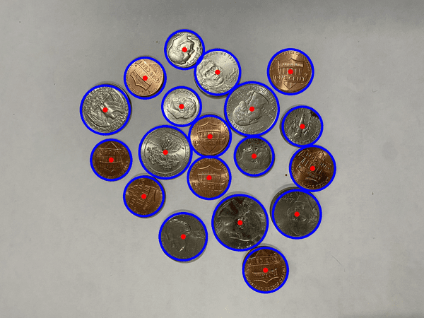
Detected circles in blue with centers in red
The code above first rounded off and converted the detected circle data into integers. Then draw the circles on the original image accordingly. From the illustration above, you can see how well the Hough Circle Transform helps you find the coins in the image.
Further Readings
P. E. Hart. “How the Hough Transform was Invented”. IEEE Signal Processing Magazine, 26(6), Nov. 2009, pp. 18–22. DOI: 10.1109/msp.2009.934181.
R. O. Duda and P. E. Hart. “Use of the Hough Transformation to Detect Lines and Curves in Pictures”. Comm. ACM, 15, Jan. 11–15. DOI: 10.1145/361237.361242.
Your Task
The detection is sensitive to the parameters you provided to \codetext{cv2.HoughCircles()} function. Try to modify the parameters and see how it results. You can also try to find the best parameters for a different picture, especially one with different lighting conditions or different resolutions.
In the next lesson, you will see how you can extract coins from the image based on the detected circles.
Lesson 04: Extracting Subimages
The image you read using OpenCV is a NumPy array of shape height×width×channel. To extract part of the image, you can simply use the NumPy slicing syntax. For example, from a BGR colored image, you can extract the red channel with:
1
red=img[:,:,2]
Therefore, to extract part of an image, you can use
1
subimg=img[y0:y1,x0:x1]
which you will get a rectangular portion of a larger image. Remember that in matrices, you first count the vertical elements (pixels) from top to bottom, then count the horizontal from left to right. Hence you should describe the $y$-coordinate range first in the slicing syntax.
Let’s modify the code in the previous lesson, to extract each coin we found:
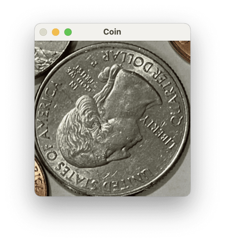
This code extracts a square subimage for each circle the Hough Transform found. Then the subimage is displayed in a window and wait for your key until the next one is displayed.
OpenCV window showing a detected coin
Your Task
Run this code. You will notice that each circle detected may be of a different size so are the subimages extracted. How can you resize the subimages to a consistent size before displaying them in the window?
In the next lesson, you will learn to compare the extracted subimages to a reference image.
With this as the reference image, how can you compare the identified coin with the reference? This is a problem more difficult than it sounds. Used coins can be rusty, dull, or with scratches. The coins in the picture can be rotated. It is not easy to compare pixels and tell if they are the same coin.
A better way is to use keypoint matching algorithms. There are several keypoint algorithms in OpenCV. Let’s try with the ORB, which is an invention from the OpenCV team. Downloading the reference image from the link above as penny.png, you can extract keypoints and keypoint descriptors with the following code:
1
2
3
4
5
6
import cv2
reference_path="penny.png"
sample=cv2.imread(reference_path)
orb=cv2.ORB_create(nfeatures=500)
kp,ref_desc=orb.detectAndCompute(sample,None)
The tuple kp are keypoint objects, but not as important as the ref_desc array, which is the keypoint descriptors. This is a NumPy array with shape $K\times 32$ for $K$ keypoints detected. Each keypoint’s ORB descriptor is a vector of 32 integers.
If you get the descriptor from another image, you can compare it to see if any keypoints match. You should not expect an exact match in descriptors. Instead, you can apply the Lowe’s ratio test to decide if the keypoints are matched:
Here, you use a brute-force matcher from cv2.BFMatcher() to run the kNN algorithm to get the two nearest neighbors from each reference keypoint to the keypoints from the candidate image. The vector distance is then compared (such that a shorter distance means a better match). The Lowe’s ratio test is to tell if the match is good enough. You may try a different constant than 0.8 above. We count the number of good matches, which we will claim the coin is identified if enough good match is found.
Below is the full code, which we will show and identify each coin found using Matplotlib. Since Matplotlib expects a colored image in RGB channels instead of BGR channels, you need to convert the image using cv2.cvtColor() before displaying it with plt.imshow().
Detected coins and the number of keypoints matched
You can see that the number of keypoints matched cannot provide a clear metric to help identify penny coins from other coins. Can you think of other algorithm other than kNN that might be helpful?
The code above uses ORB keypoints. You can also try with SIFT keypoints. How to modify the code above? Would you see the change in the number of keypoints matched? Also, since ORB features are vectors. Can you build a logistic regression classifier to identify good keypoints such that you do not need to rely on a reference image?
In the next lesson, you will work on a better coin identifier.
Lesson 06: Building a Coin Classifier
Provided with an image of a coin and identifying if it is a U.S. penny coin is easy for humans but not so for computers. It is known that the best way to do such classification is by machine learning. You should first extract feature vectors from the image, then run a machine learning algorithm as a classifier to tell if it is a match or not.
Deciding which feature to use is a hard problem itself. But if you use the convolutional neural network, you can let the machine learning algorithm figure out the features by itself. But to train a neural network, you need data. Fortunately, you don’t need a lot. Let’s see how you can build one.
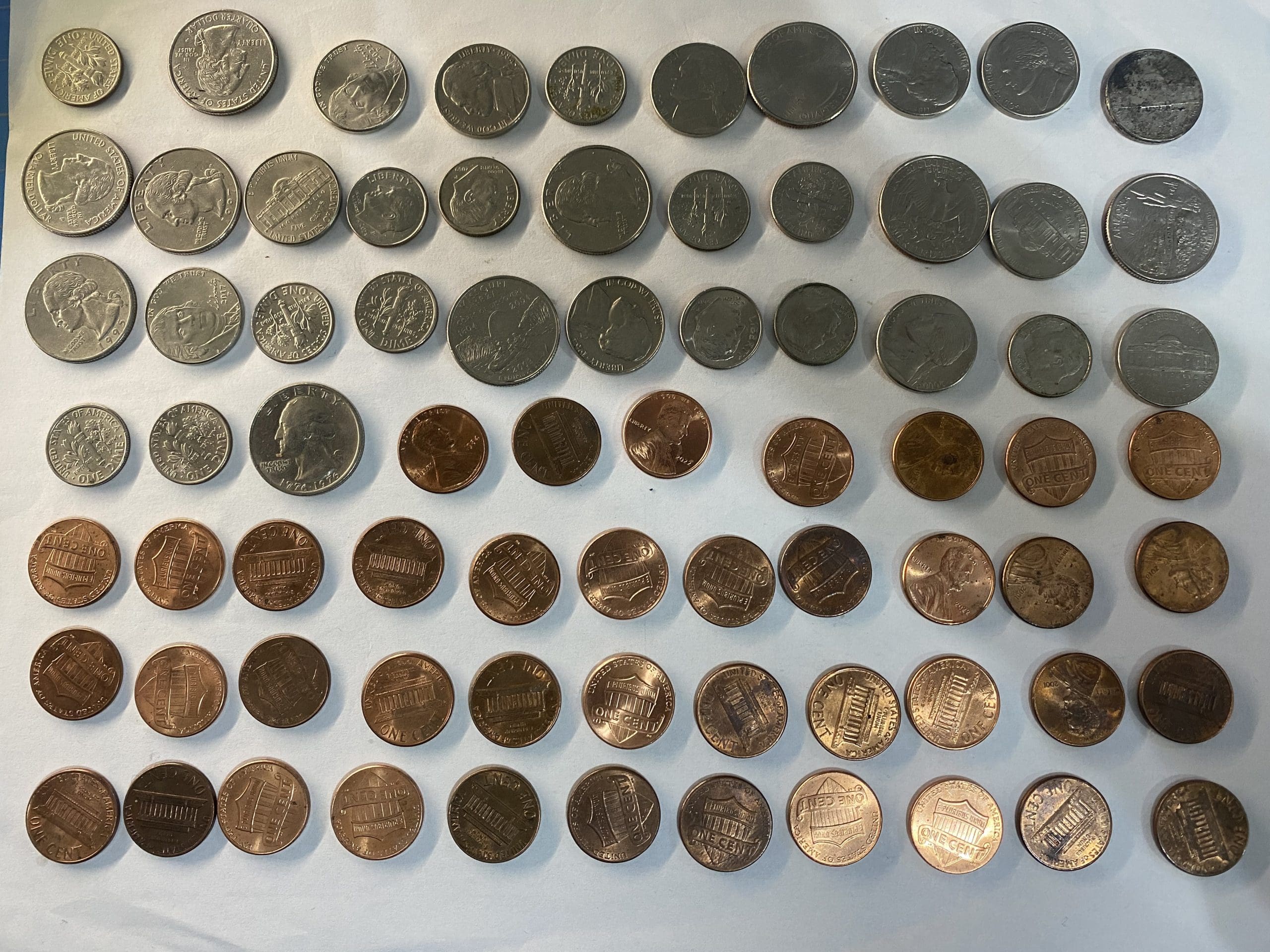
Firstly, you can get a picture of some coins here:
There are not many images. You can manually tag each image as a penny coin (positive) or not (negative). One way is to move the positive samples into the sub-directory dataset/pos and the negative samples into dataset/neg. For your convenience, you can find a copy of tagged images in the zip file here.
With these, let’s build a convolutional neural network for this binary classification problem, using Keras and TensorFlow.
During the data preparation phase, you will read each positive and negative image sample. To make the convolutional neural network simpler, you fixed the input size to $256\times 256$ pixels by resizing the image first. To increase variations in the dataset, you can rotate each image by 90, 180, and 270 degrees and add to the dataset (it is easy since the image samples are all square). Then, you can make use of the train_test_split() function from scikit-learn to separate the dataset into training and test sets in a ratio of 7:3.
To create the model, you can use the classific architecture of multiple Conv2D layers with MaxPooling, then followed by Dense layers at the output. Note that it is a binary classification model. Hence at the final output layer, you should use sigmoid activation.
At training, you can simply use a large number of iterations (e.g., epochs=200) with early stopping so you don’t need to worry about underfitting. You should monitor for the loss evaluated at the test set to be sure not to run into overfitting. In code, this is how you can train a model and save the model as penny.h5:
1
2
3
4
5
6
7
8
9
10
11
12
13
14
15
16
17
18
19
20
21
22
23
24
25
26
27
28
29
30
31
32
33
34
35
36
37
38
39
40
41
42
43
44
45
46
47
48
49
50
51
52
import glob
import cv2
import numpy asnp
from sklearn.model_selection import train_test_split
from tensorflow.keras.callbacks import EarlyStopping
from tensorflow.keras.layers import Conv2D,Dense,MaxPooling2D,Flatten
Observe its output, you should easily see the accuracy reach above 90% with not many iterations.
Your Task
Run the code above and create a trained model in penny.h5, which you will use in the next lesson.
You can modify the model design and see if you can improve the accuracy. Some ideas you can try are: using a different number of Conv2D-MaxPooling layers, different sizes of each layer other than 16-32-64-128 above, or using an activation function other than ReLU.
In the next lesson, you will convert the model you created in Keras to use in OpenCV.
Lesson 07: Using DNN Module in OpenCV
Given you have built a convolutional neural network in the previous lesson, you can now use it together with OpenCV. It is easier for OpenCV to consume your model if you first convert it into ONNX format. To do so, you would need the tf2onnx module from Python. Once you installed it, you can convert the model with the following command:
As you saved your Keras model as penny.h5, this command will create the file penny.onnx.
With the ONNX model file, you can now use the cv2.dnn module from OpenCV. The usage is as follows:
1
2
3
4
5
import cv2
net=cv2.dnn.readNetFromONNX("penny.onnx")
net.setInput(blob)
output=float(net.forward())
That is, you create a neural network object with OpenCV, assign the input, and run the model with forward() to fetch the output, which according to how you designed your model, is a floating point value between 0 and 1. As a convention in neural networks, the input is batched even if you provide only one input sample. Hence you should add a batch dimension to the images before sending them to the neural network.
Now let’s see how you can achieve the goal of counting pennies. You can start by modifying the code from Lesson 05, as follows:
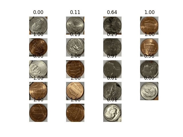
Instead of using ORB and counting the good keypoints for a match, you used the convolutional neural network to read the sigmoidal output. The output is as follows:
Detected coins and the match score by the neural network
You can see quite good a result with this model. All the pennies are identified with a score close to 1. The negative samples are not as good (probably because we did not provide enough negative samples). Let’s use 0.9 as the score cut-off value and rewrite the program to give a count:
Can you modify the code above to report the count by reading images continuously from your webcam?
This was the final lesson.
The End! (Look How Far You Have Come)
You made it. Well done!
Take a moment and look back at how far you have come.
You discovered OpenCV as a machine learning library in addition to its image processing capabilities.
You made use of OpenCV to extract image features as numerical vectors, which is the basis for any machine learning algorithm.
You built a neural network model and converted it to use with OpenCV.
Finally, you build a penny counter program. While not perfect, it demonstrates how you can combine OpenCV with machine learning.
Don’t make light of this, you have come a long way in a short amount of time. This is just the beginning of your computer vision journey with machine learning. Keep practicing and developing your skills.
Summary
How did you do with the mini-course?
Did you enjoy this crash course?
Do you have any questions? Were there any sticking points?
Let me know. Leave a comment below.
Get Started on Machine Learning in OpenCV!
Learn how to use machine learning techniques in image processing projects
...using OpenCV in advanced ways and work beyond pixels
It provides self-study tutorials with all working code in Python to turn you from a novice to expert. It equips you with logistic regression, random forest, SVM, k-means clustering, neural networks,
and much more...all using the machine learning module in OpenCV
Kick-start your deep learning journey with hands-on exercises


")
")
")
")
")
")
No comments yet.