Deep Learning with PyTorch (9-Day Mini-Course)

By Adrian Tam on January 22, 2024 in Deep Learning with PyTorch 13

Deep learning is a fascinating field of study and the techniques are achieving world class results in a range of challenging machine learning problems. It can be hard to get started in deep learning.
Which library should you use and which techniques should you focus on?

In this 9-part crash course you will discover applied deep learning in Python with the easy to use and powerful PyTorch library. This mini-course is intended for practitioners that are already comfortable with programming in Python and knows the basic concept of machine learning. Let’s get started.

This is a long and useful post. You might want to print it out.

Let’s get started.

Deep Learning with PyTorch (9-day Mini-Course)
Photo by Cosmin Georgian. Some rights reserved.

Who Is This Mini-Course For?

Before we get started, let’s make sure you are in the right place. The list below provides some general guidelines as to who this course was designed for. Don’t panic if you don’t match these points exactly, you might just need to brush up in one area or another to keep up.

Developers that know how to write a little code. This means that it is not a big deal for you to get things done with Python and know how to setup the ecosystem on your workstation (a prerequisite). It does not mean you’re a wizard coder, but it does mean you’re not afraid to install packages and write scripts.
Developers that know a little machine learning. This means you know about the basics of machine learning like cross-validation, some algorithms and the bias-variance trade-off. It does not mean that you are a machine learning PhD, just that you know the landmarks or know where to look them up.

This mini-course is not a textbook on Deep Learning.

It will take you from a developer that knows a little machine learning in Python to a developer who can get results and bring the power of Deep Learning to your own projects.

Mini-Course Overview

This mini-course is divided into 9 parts.

Each lesson was designed to take the average developer about 30 minutes. You might finish some much sooner and other you may choose to go deeper and spend more time.
You can complete each part as quickly or as slowly as you like. A comfortable schedule may be to complete one lesson per day over nine days. Highly recommended.

The topics you will cover over the next 9 lessons are as follows:

Lesson 1: Introduction to PyTorch.
Lesson 2: Build Your First Multilayer Perceptron Model
Lesson 3: Training a PyTorch Model
Lesson 4: Using a PyTorch Model for Inference
Lesson 5: Loading Data from Torchvision
Lesson 6: Using PyTorch DataLoader
Lesson 7: Convolutional Neural Network
Lesson 8: Train an Image Classifier
Lesson 9: Train with GPU

This is going to be a lot of fun.

You’re going to have to do some work though, a little reading, a little research and a little programming. You want to learn deep learning right?

Post your results in the comments; I’ll cheer you on!

Hang in there; don’t give up.

Lesson 01: Introduction to PyTorch

PyTorch is a Python library for deep learning computing created and released by Facebook. It has its root from an earlier library Torch 7 but completely rewritten.

It is one of the two most popular deep learning libraries. PyTorch is a complete library that has the capability to train a deep learning model as well as run a model in inference mode, and supports using GPU for faster training and inference. It is a platform that we cannot ignore.

In this lesson your goal is to install PyTorch become familiar with the syntax of the symbolic expressions used in PyTorch programs.
For example, you can install PyTorch using pip. The latest version of PyTorch at the time of writing is 2.0. There are PyTorch prebuilt for each platform, including Windows, Linux, and macOS. With a working Python environment, pip should take care of that for you to provide you the latest version in your platform.

Besides PyTorch, there is also the torchvision library that is commonly used together with PyTorch. It provides a lot of useful functions to help computer vision projects.

sudo pip install torch torchvision

1	sudo pip install torch torchvision

A small example of a PyTorch program that you can use as a starting point is listed below:

# Example of PyTorch library
import torch
# declare two symbolic floating-point scalars
a = torch.tensor(1.5)
b = torch.tensor(2.5)
# create a simple symbolic expression using the add function
c = torch.add(a, b)
print(c)

# Example of PyTorch library

import torch

# declare two symbolic floating-point scalars

a = torch.tensor(1.5)

b = torch.tensor(2.5)

# create a simple symbolic expression using the add function

c = torch.add(a, b)

print(c)

Learn more about PyTorch on the PyTorch homepage.

Your Task

Repeat the above code to make sure you have PyTorch correctly installed. You can also check your PyTorch version by running the following lines of Python code:

import torch
print(torch.__version__)

1 2	import torch print(torch.__version__)

In the next lesson, you will use PyTorch to build a neural network model.

Lesson 02: Build Your First Multilayer Perceptron Model

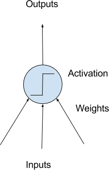
Deep learning is about building large scale neural networks. The simplest form of neural network is called multilayer perceptron model. The building block for neural networks are artificial neurons or perceptrons. These are simple computational units that have weighted input signals and produce an output signal using an activation function.

Perceptrons are arranged into networks. A row of perceptrons is called a layer and one network can have multiple layers. The architecture of the perceptrons in the network is often called the network topology. Once configured, the neural network needs to be trained on your dataset. The classical and still preferred training algorithm for neural networks is called stochastic gradient descent.

Model of a Simple Neuron

PyTorch allows you to develop and evaluate deep learning models in very few lines of code.

In the following, your goal is to develop your first neural network using PyTorch. Use a standard binary (two-class) classification dataset from the UCI Machine Learning Repository, like the Pima Indians dataset.

To keep things simple, the network model is just a few layers of fully-connected perceptrons. In this particular model, the dataset has 12 inputs or predictors and the output is a single value of 0 or 1. Therefore, the network model should have 12 inputs (at the first layer) and 1 output (at the last layer). Your first model would be built as follows:

import torch.nn as nn

model = nn.Sequential(
  nn.Linear(8, 12),
  nn.ReLU(),
  nn.Linear(12, 8),
  nn.ReLU(),
  nn.Linear(8, 1),
  nn.Sigmoid()
)
print(model)

import torch.nn as nn

model = nn.Sequential(

nn.Linear(8, 12),

nn.ReLU(),

nn.Linear(12, 8),

nn.ReLU(),

nn.Linear(8, 1),

nn.Sigmoid()

)

print(model)

This is a network with 3 fully-connected layers. Each layer is created in PyTorch using the nn.Linear(x, y) syntax which the first argument is the number of input to the layer and the second is the number of output. Between each layer, a rectified linear activation is used, but at the output, sigmoid activation is applied such that the output value is between 0 and 1. This is a typical network. A deep learning model is to have a lot of such layers in a model.

Your Task

Repeat the above code and observe the printed model output. Try to add another layer that outputs 20 values after the first Linear layer above. What should you change to the line of nn.Linear(12, 8) to accommodate this addition?

In the next lesson, you will see how to train this model.

Lesson 03: Training a PyTorch Model

Building a neural network in PyTorch does not tell how you should train the model for a particular job. In fact, there are many variations in this aspect as described by the hyperparameters. In PyTorch, or all deep learning models in general, you need to decide the following on how to train a model:

What is the dataset, specifically how the input and target looks like
What is the loss function to evaluate the goodness of fit of the model to the data
What is the optimization algorithm to train the model, and the parameters to the optimization algorithm such as learning rate and number of
iterations to train

In the previous lesson, the Pima Indian dataset is used and all the input are numbers. This would be the simplest case as you are not required to do any preprocessing of the data since neural networks can readily handle numbers.

Since it is a binary classification problem, the loss function should be binary cross entropy. It means that the target of the model output is 0 or 1 for the classification result. But in reality the model may output anything in between. The closer it is to the target value, the better (i.e., lower loss).

Gradient descent is the algorithm to optimize neural networks. There are many variations of gradient descent and Adam is one of the most used.

Implementing all the above, together with the model built in the previous lesson, the following is the code of the training process:

import numpy as np
import torch
import torch.nn as nn
import torch.optim as optim

dataset = np.loadtxt('pima-indians-diabetes.csv', delimiter=',')
X = dataset[:,0:8]
y = dataset[:,8]
X = torch.tensor(X, dtype=torch.float32)
y = torch.tensor(y, dtype=torch.float32).reshape(-1, 1)

loss_fn = nn.BCELoss() # binary cross-entropy
optimizer = optim.Adam(model.parameters(), lr=0.001)

n_epochs = 100
batch_size = 10
for epoch in range(n_epochs):
    for i in range(0, len(X), batch_size):
        Xbatch = X[i:i+batch_size]
        y_pred = model(Xbatch)
        ybatch = y[i:i+batch_size]
        loss = loss_fn(y_pred, ybatch)
        optimizer.zero_grad()
        loss.backward()
        optimizer.step()
    print(f'Finished epoch {epoch}, latest loss {loss}')

import numpy as np

import torch

import torch.nn as nn

import torch.optim as optim

dataset = np.loadtxt('pima-indians-diabetes.csv', delimiter=',')

X = dataset[:,0:8]

y = dataset[:,8]

X = torch.tensor(X, dtype=torch.float32)

y = torch.tensor(y, dtype=torch.float32).reshape(-1, 1)

loss_fn = nn.BCELoss() # binary cross-entropy

optimizer = optim.Adam(model.parameters(), lr=0.001)

n_epochs = 100

batch_size = 10

for epoch in range(n_epochs):

for i in range(0, len(X), batch_size):

Xbatch = X[i:i+batch_size]

y_pred = model(Xbatch)

ybatch = y[i:i+batch_size]

loss = loss_fn(y_pred, ybatch)

optimizer.zero_grad()

loss.backward()

optimizer.step()

print(f'Finished epoch {epoch}, latest loss {loss}')

The for-loop above is to get a batch of data and feed into the model. Then observe the model’s output and calculate the loss function. Based on the loss function, the optimizer will fine-tune the model for one step, so it can match better to the training data. After a number of update steps, the model should be close enough to the training data that it can predict the target at a high accuracy.

Your Task

Run the training loop above and observe how the loss decreases as the training loop proceeds.

In the next lesson, you will see how use the trained model.

Lesson 04: Using a PyTorch Model for Inference

A trained neural network model is a model that remembered how the input and target related. Then, this model can predict the target given another input.

In PyTorch, a trained model can behave just like a function. Assume you have the model trained in the previous lesson, you can simply use it as follows:

i = 5
X_sample = X[i:i+1]
y_pred = model(X_sample)
print(f"{X_sample[0]} -> {y_pred[0]}")

i = 5

X_sample = X[i:i+1]

y_pred = model(X_sample)

print(f"{X_sample[0]} -> {y_pred[0]}")

But in fact, the better way of running inference is the following:

i = 5
X_sample = X[i:i+1]
model.eval()
with torch.no_grad():
    y_pred = model(X_sample)
print(f"{X_sample[0]} -> {y_pred[0]}")

i = 5

X_sample = X[i:i+1]

model.eval()

with torch.no_grad():

y_pred = model(X_sample)

print(f"{X_sample[0]} -> {y_pred[0]}")

Some model will behave differently between training and inference. The line of model.eval() is to signal the model that the intention is to run the model for inference. The line with torch.no_grad() is to create a context for running the model, such that PyTorch knows calculating the gradient is not required. This can consume less resources.

This is also how you can evaluate the model. The model outputs a sigmoid value, which is between 0 and 1. You can interpret the value by rounding off the value to the closest integer (i.e., Boolean label). Comparing how often the prediction after round off match the target, you can assign an accuracy percentage to the model, as follows:

model.eval()
with torch.no_grad():
    y_pred = model(X)
accuracy = (y_pred.round() == y).float().mean()
print(f"Accuracy {accuracy}")

model.eval()

with torch.no_grad():

y_pred = model(X)

accuracy = (y_pred.round() == y).float().mean()

print(f"Accuracy {accuracy}")

Your Task

Run the above code and see what is the accuracy you get. You should achieve roughly 75%.

In the next lesson, you will learn about torchvision.

Lesson 05: Loading Data from Torchvision

Torchvision is a sister library to PyTorch. In this library, there are functions specialized for image and computer vision. As you can expect, there are functions to help you read images or adjust the contrast. But probably most important is to provide an easy interface to get some image datasets.

In the next lesson, you will build a deep learning model to classify small images. This is a model that allows your computer to see what’s on an image. As you saw in the previous lessons, it is important to have the dataset to train the model. The dataset you’re going to use is CIFAR-10. It is a dataset of 10 different objects. There is a larger dataset called CIFAR-100, too.

The CIFAR-10 dataset can be downloaded from the Internet. But if you have torchvision installed, you just need to do the following:

import matplotlib.pyplot as plt
import torchvision

trainset = torchvision.datasets.CIFAR10(root='./data', train=True, download=True)
testset = torchvision.datasets.CIFAR10(root='./data', train=False, download=True)

fig, ax = plt.subplots(4, 6, sharex=True, sharey=True, figsize=(12,8))
for i in range(0, 24):
    row, col = i//6, i%6
    ax[row][col].imshow(trainset.data[i])
plt.show()

import matplotlib.pyplot as plt

import torchvision

trainset = torchvision.datasets.CIFAR10(root='./data', train=True, download=True)

testset = torchvision.datasets.CIFAR10(root='./data', train=False, download=True)

fig, ax = plt.subplots(4, 6, sharex=True, sharey=True, figsize=(12,8))

for i in range(0, 24):

row, col = i//6, i%6

ax[row][col].imshow(trainset.data[i])

plt.show()

The torchvision.datasets.CIFAR10 function helps you to download the CIFAR-10 dataset to a local directory. The dataset is divided into training set and test set. Therefore the two lines above is to get both of them. Then you plot the first 24 images from the downloaded dataset. Each image in the dataset is 32×32 pixels picture of one of the following: airplane, automobile, bird, cat, deer, dog, frog, horse, ship, or truck.

Your Task

Based on the code above, can you find a way to count how many images in total in the training set and test set, respectively?

In the next lesson, you will learn how to use PyTorch DataLoader.

Lesson 06: Using PyTorch DataLoader

The CIFAR-10 image from the previous lesson is indeed in the format of numpy array. But for consumption by a PyTorch model, it needs to be in PyTorch tensors. It is not difficult to convert a numpy array into PyTorch tensor but in the training loop, you still need to divide the dataset in batches. The PyTorch DataLoader can help you make this process smoother.

Back to the CIFAR-10 dataset as loaded in the previous lesson, you can do the following for the identical effect:

import matplotlib.pyplot as plt
import torchvision
import torch
from torchvision.datasets import CIFAR10

transform = torchvision.transforms.Compose([torchvision.transforms.ToTensor()])
trainset = CIFAR10(root='./data', train=True, download=True, transform=transform)
testset = CIFAR10(root='./data', train=False, download=True, transform=transform)

batch_size = 24
trainloader = torch.utils.data.DataLoader(trainset, batch_size=batch_size, shuffle=True)
testloader = torch.utils.data.DataLoader(testset, batch_size=batch_size, shuffle=True)

fig, ax = plt.subplots(4, 6, sharex=True, sharey=True, figsize=(12,8))
for images, labels in trainloader:
    for i in range(batch_size):
        row, col = i//6, i%6
        ax[row][col].imshow(images[i].numpy().transpose([1,2,0]))
    break  # take only the first batch
plt.show()

import matplotlib.pyplot as plt

import torchvision

import torch

from torchvision.datasets import CIFAR10

transform = torchvision.transforms.Compose([torchvision.transforms.ToTensor()])

trainset = CIFAR10(root='./data', train=True, download=True, transform=transform)

testset = CIFAR10(root='./data', train=False, download=True, transform=transform)

batch_size = 24

trainloader = torch.utils.data.DataLoader(trainset, batch_size=batch_size, shuffle=True)

testloader = torch.utils.data.DataLoader(testset, batch_size=batch_size, shuffle=True)

fig, ax = plt.subplots(4, 6, sharex=True, sharey=True, figsize=(12,8))

for images, labels in trainloader:

for i in range(batch_size):

row, col = i//6, i%6

ax[row][col].imshow(images[i].numpy().transpose([1,2,0]))

break # take only the first batch

plt.show()

In this code, trainset is created with transform argument so that the data is converted into PyTorch tensor when it is extracted. This is performed in DataLoader the lines following it. The DataLoader object is a Python iterable, which you can extract the input (which are images) and target (which are integer class labels). In this case, you set the batch size to 24 and iterate for the first batch. Then you show each image in the batch.

Your Task

Run the code above and compare with the matplotlib output you generated in the previous lesson. You should see the output are different. Why? There is an argument in the DataLoader lines caused the difference. Can you identify which one?

In the next lesson, you will learn how to build a deep learning model to classify the images from CIFAR-10 dataset.

Lesson 07: Convolutional Neural Network

Images are 2D structures. You can easily convert them into 1D vectors by flattening it and build a neural network model to classify them. But it is known that preserving the 2D structure would be more appropriate because the classification is about what’s in the image, which is translation invariant.

The standard way for image processing neural network is to use convolutional layers. A neural network that uses convolutional layers is called a convolutional neural network. An example is as follows:

import torch.nn as nn

model = nn.Sequential(
    nn.Conv2d(3, 32, kernel_size=(3,3), stride=1, padding=1),
    nn.ReLU(),
    nn.Dropout(0.3),
    nn.Conv2d(32, 32, kernel_size=(3,3), stride=1, padding=1),
    nn.ReLU(),
    nn.MaxPool2d(kernel_size=(2, 2)),
    nn.Flatten(),
    nn.Linear(8192, 512),
    nn.ReLU(),
    nn.Dropout(0.5),
    nn.Linear(512, 10)
)
print(model)

import torch.nn as nn

model = nn.Sequential(

nn.Conv2d(3, 32, kernel_size=(3,3), stride=1, padding=1),

nn.ReLU(),

nn.Dropout(0.3),

nn.Conv2d(32, 32, kernel_size=(3,3), stride=1, padding=1),

nn.ReLU(),

nn.MaxPool2d(kernel_size=(2, 2)),

nn.Flatten(),

nn.Linear(8192, 512),

nn.ReLU(),

nn.Dropout(0.5),

nn.Linear(512, 10)

)

print(model)

In the above, we used Conv2d layers several times, as well as ReLU activation. The convolutional layers are to learn and extract features from image. More convolutional layers you add, the network can learn more high-level features. Eventually, you would use a pooling layer (MaxPool2d above) to group the extracted features, flatten them into a vector, then pass it on to a multilayer perceptron network for final classification. This is the usual structure of an image classification model.

Your Task

Run the above code to make sure you can correctly create a model. You didn’t specify the input image size in the model but indeed it is fixed to 32×32 pixels in RGB (i.e., 3 color channels). Where is this fixed in the network?

In the next lesson, you will use the DataLoader in the previous lesson to train the model above.

Lesson 08: Train an Image Classifier

Together with the DataLoader created for CIFAR-10 dataset, you can train the convolutional neural network in the previous lesson with the following training loop:

import torch.nn as nn
import torch.optim as optim

loss_fn = nn.CrossEntropyLoss()
optimizer = optim.SGD(model.parameters(), lr=0.001, momentum=0.9)

n_epochs = 20
for epoch in range(n_epochs):
    model.train()
    for inputs, labels in trainloader:
        y_pred = model(inputs)
        loss = loss_fn(y_pred, labels)
        optimizer.zero_grad()
        loss.backward()
        optimizer.step()
    acc = 0
    count = 0
    model.eval()
    with torch.no_grad():
        for inputs, labels in testloader:
            y_pred = model(inputs)
            acc += (torch.argmax(y_pred, 1) == labels).float().sum()
            count += len(labels)
    acc /= count
    print("Epoch %d: model accuracy %.2f%%" % (epoch, acc*100))

import torch.nn as nn

import torch.optim as optim

loss_fn = nn.CrossEntropyLoss()

optimizer = optim.SGD(model.parameters(), lr=0.001, momentum=0.9)

n_epochs = 20

for epoch in range(n_epochs):

model.train()

for inputs, labels in trainloader:

y_pred = model(inputs)

loss = loss_fn(y_pred, labels)

optimizer.zero_grad()

loss.backward()

optimizer.step()

acc = 0

count = 0

model.eval()

with torch.no_grad():

for inputs, labels in testloader:

y_pred = model(inputs)

acc += (torch.argmax(y_pred, 1) == labels).float().sum()

count += len(labels)

acc /= count

print("Epoch %d: model accuracy %.2f%%" % (epoch, acc*100))

This will take a while to run, and you should see the model produced can achieve no less than 70% accuracy.

This model is a multiclass classification network. The output is not one, but many scores, one for each class. We consider the higher score the more confident the model thinks the image belongs to a class. The loss function used is therefore cross-entropy, the multiclass version of binary cross-entropy.

In the training loop above, you should see quite many elements you learned in the previous lessons. Including switching between training and inference mode in the model, using torch.no_grad() context, and calculation of the accuracy.

Your Task

Read the code above to make sure you understand what it does. Run this code to observe the accuracy increase as the training proceeds. What is the final accuracy you achieved?

In the next lesson, you will learn how to use GPU to speed up the training of the same model.

Lesson 09: Train with GPU

The model training you did in the previous lesson should take a while. If you have a supported GPU, you can speed up the training a lot.

The way to use GPU in PyTorch is to send the model and data to GPU before execution. Then you have an option to send back the result from GPU, or perform the evaluation in GPU directly.

It is not difficult to modify the code from the previous lesson to use GPU. Below is what it should be done:

import torch.nn as nn
import torch.optim as optim

device = torch.device("cuda:0" if torch.cuda.is_available() else "cpu")
model.to(device)

loss_fn = nn.CrossEntropyLoss()
optimizer = optim.SGD(model.parameters(), lr=0.001, momentum=0.9)

n_epochs = 20
for epoch in range(n_epochs):
    model.train()
    for inputs, labels in trainloader:
        y_pred = model(inputs.to(device))
        loss = loss_fn(y_pred, labels.to(device))
        optimizer.zero_grad()
        loss.backward()
        optimizer.step()
    acc = 0
    count = 0
    model.eval()
    with torch.no_grad():
        for inputs, labels in testloader:
            y_pred = model(inputs.to(device))
            acc += (torch.argmax(y_pred, 1) == labels.to(device)).float().sum()
            count += len(labels)
    acc /= count
    print("Epoch %d: model accuracy %.2f%%" % (epoch, acc*100))

import torch.nn as nn

import torch.optim as optim

device = torch.device("cuda:0" if torch.cuda.is_available() else "cpu")

model.to(device)

loss_fn = nn.CrossEntropyLoss()

optimizer = optim.SGD(model.parameters(), lr=0.001, momentum=0.9)

n_epochs = 20

for epoch in range(n_epochs):

model.train()

for inputs, labels in trainloader:

y_pred = model(inputs.to(device))

loss = loss_fn(y_pred, labels.to(device))

optimizer.zero_grad()

loss.backward()

optimizer.step()

acc = 0

count = 0

model.eval()

with torch.no_grad():

for inputs, labels in testloader:

y_pred = model(inputs.to(device))

acc += (torch.argmax(y_pred, 1) == labels.to(device)).float().sum()

count += len(labels)

acc /= count

print("Epoch %d: model accuracy %.2f%%" % (epoch, acc*100))

The changes made are the following: You check if GPU is available and set the device accordingly. Then the model is sent to the device. When the input (i.e., a batch of images) is pass on to the model, it should be sent to the corresponding device first. Since the model output will also be there, the loss calculation or the accuracy calculation should also have the target sent to the GPU first.

Your Task

You can see the running PyTorch in CPU and in GPU are mostly the same. Try compare the two if you can access to a GPU. How much faster you can observe?

This was the final lesson.

The End! (Look How Far You Have Come)

You made it. Well done!

Take a moment and look back at how far you have come.

You discovered PyTorch as a deep learning library in Python
You built your first neural network using PyTorch and learned how to do classification with a neural network
You learned key components in deep learning, including loss function, optimizer, training loop, and evaluation
Finally, you took the next step and learned about and developed convolutional neural networks for computer vision tasks

Summary

How did you do with the mini-course?
Did you enjoy this crash course?

Do you have any questions? Were there any sticking points?
Let me know. Leave a comment below.

13 Responses to Deep Learning with PyTorch (9-Day Mini-Course)

ayush April 10, 2023 at 8:02 pm #

Thank you for the valuable information on the blog.
I am not an expert in blog writing, but I am reading your content slightly, increasing my confidence in how to give the information properly. Your presentation was also good, and I understood the information easily.

- James Carmichael April 11, 2023 at 6:08 am #
  
  You are very welcome ayush! We greatly appreciate your feedback and support!
  
Aashi Goel May 5, 2023 at 2:58 pm #

I was looking for something just like this! Thanks a lot for this mini-course, I can’t wait to start this.

Jamina A May 5, 2023 at 4:29 pm #

Hi, thanks for the post.

In lesson 2, you have mentioned 12 inputs, but the code at line 4 is:

nn.Linear(8, 12)

Since the 1 st parameter is input, should it be
nn.Linear(12,8). ?

Thanks

- James Carmichael May 6, 2023 at 10:26 am #
  
  Hi Jamina…You are correct! Thank you for your feedback!
  
Chase He May 22, 2023 at 11:30 am #

Nice course! Can you comment on how to increase accuracy? like changing learning rate? Increase model layer or change layer size?

- James Carmichael May 23, 2023 at 6:09 am #
  
  Hi Chase He…We appreciate your feedback! The following resource addresses many techniques to improve performance:
  
  https://machinelearningmastery.com/better-deep-learning/
  
Chase He May 22, 2023 at 11:31 am #

Nice course! Can you comment on how to increase accuracy? like changing the learning rate? Increase model layer or change layer size?

AmerAther October 24, 2023 at 7:17 am #

In lesson2, I am getting error:
”
Traceback (most recent call last):
File “./lesson2.py”, line 14, in
optimizer = optim.Adam(model.parameters(), lr=0.001)
NameError: name ‘model’ is not defined”

- James Carmichael October 24, 2023 at 10:08 am #
  
  Hi AmerAther…Did you type the code in or copy and past it?
  
AmerAther October 24, 2023 at 7:23 am #

I found the issue. Please ignore

Jay December 30, 2023 at 2:27 am #

Hi,
After running Day 2 code, giving below output only. Ideally it should give details. Is this settings issue or ? Please help.

Sequential(
(0): Linear(in_features=8, out_features=12, bias=True)
(1): ReLU()
(2): Linear(in_features=12, out_features=8, bias=True)
(3): ReLU()
(4): Linear(in_features=8, out_features=1, bias=True)
(5): Sigmoid()
)

- James Carmichael December 30, 2023 at 9:32 am #
  
  Hi Jay…Please elaborate on the exact verbiage of the errors you are encountering so that we may better assist you.

Navigation

Deep Learning with PyTorch (9-Day Mini-Course)

Who Is This Mini-Course For?

Mini-Course Overview

Lesson 01: Introduction to PyTorch

Your Task

Lesson 02: Build Your First Multilayer Perceptron Model

Your Task

Lesson 03: Training a PyTorch Model

Your Task

Lesson 04: Using a PyTorch Model for Inference

Your Task

Lesson 05: Loading Data from Torchvision

Your Task

Lesson 06: Using PyTorch DataLoader

Your Task

Lesson 07: Convolutional Neural Network

Your Task

Lesson 08: Train an Image Classifier

Your Task

Lesson 09: Train with GPU

Your Task

The End! (Look How Far You Have Come)

Summary

Get Started on Deep Learning with PyTorch!

Learn how to build deep learning models

Kick-start your deep learning journey with hands-on exercises

More On This Topic

13 Responses to Deep Learning with PyTorch (9-Day Mini-Course)

Leave a Reply Click here to cancel reply.