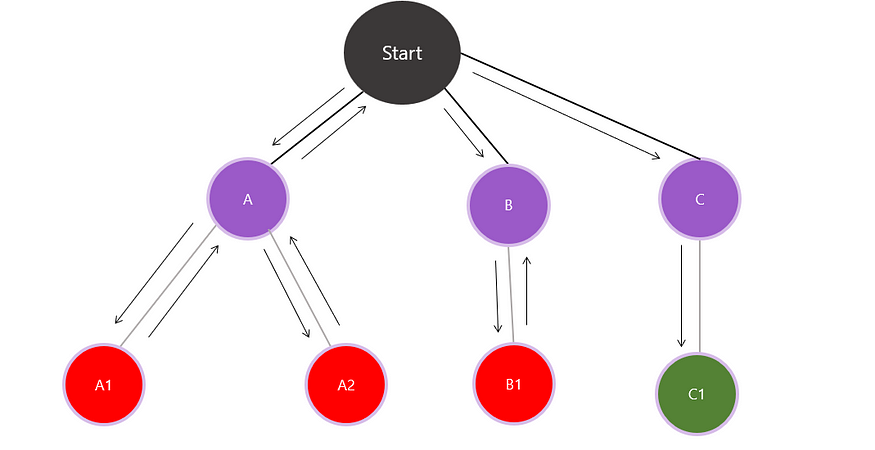
Understanding Backtracking using Python: Beginners Guide

Author(s): Muttineni Sai Rohith

Originally published on Towards AI.

Backtracking is an algorithm used to search for all possible solutions to a problem. In this technique, we find a solution to a problem by incrementally building a solution and undoing it when it is not correct or when all the possibilities are explored. It is commonly used in problems where there is a chance of one or more valid solutions to a problem. Backtracking is often implemented using recursion.

Types of Backtracking:

While backtracking can be used to solve problems such as Decision problems, optimization problems, and Enumeration problems, there are different types of Backtracking —

• Recursive Backtracking: Backtracking is often implemented using recursive functions, with each recursive call representing a decision. In a few cases, iterative backtracking is used, using stacks and queues to keep track of decisions.
• Optimization Backtracking: In a few problems, Backtracking is used not only to find all possible solutions but also to find the best solution among the possibilities. This involves pruning techniques to eliminate calls that cannot lead to optimal solutions. Sometimes, Backtracking can also be coupled with memoization and tabulation in Dynamic Programming.
• Heuristic Backtracking: This kind of backtracking is mostly used in AI. In the case of exhaustive exploration space, heuristics can be used to guide the backtracking algorithm towards finding an optimal solution.

Approach:

First, we form a state tree, as shown in the above diagram, which comprises different states to solve a given problem. Then, we traverse through each state to identify whether it can be a solution or leads to a solution, and then, depending on the outcome, we can make the decision to discard all the invalid solutions in that iteration.

Let's learn how to do Backtracking in Python by going through a few examples:

1. Find all subsets of a given array

Given an integer array nums of unique elements, return all possible subsets (the power set).

The solution set must not contain duplicate subsets. Return the solution in any order

Example 1:

Input: nums = [1,2,3]
Output: [[],[1],[2],[1,2],[3],[1,3],[2,3],[1,2,3]]

Example 2:

Input: nums = [0]
Output: [[],[0]]

Code:

class Solution:
 def subsets(self, nums: List[int]) -> List[List[int]]:
 result, subset, = [], []
 result = self.retrieve_subsets(nums, result, subset, 0)
 return result
 
 def retrieve_subsets(self, nums, result, subset, index):
 result.append(subset[:])
 for i in range(index, len(nums)):
 subset.append(nums[i])
 self.retrieve_subsets(nums, result, subset, i+1)
 subset.pop()
 return result

Explanation:

* Let's start execution by taking an Initial array - [1,2,3]
* Initial State
 - Array(nums) = [1,2,3]
 - result = []
 - subset = []
 - index = 0
* State - 1 [Initial Function Call]
 - Result: result = [[]]
* State - 2 [Recursive Call with Index = 0]
 - index = 0
 - subset = [1]
 - recursive call is made with the updated subset and index = 1
* State - 3 [Recursive Call with Index = 1]
 - index = 1
 - subset = [1,2]
 - recursive call is made with the updated subset and index = 2
* State - 4[Recursive Call with Index = 2]
 - index = 2
 - subset = [1,2,3]
 - recursive call is made with the updated subset, as there are no elements,
 loop terminates
* State - 5[Backtracking to Index = 1]
 - Backtrack to previous recursive call where index = 1
 - Pop the last element from subset, subset = [1,2]
 - The loop proceeds to the next iteration, i = 2,
 adding Arr[2] to the subset, making subset = [1, 2, 3].
* State - 6[Backtracking to Index = 0]
 - Backtrack to previous recursive call where index = 1
 - Pop the last element from subset, subset = [1]
 - The loop proceeds to the next iteration, i = 1,
 adding Arr[1] to the subset, making subset = [1, 3].
and the process continues untill all the possible states are explored.
Result: result = [[], [1], [1, 2], [1, 2, 3], [1, 3], [2], [2, 3], [3]]

2. All Paths From Source to Target

Given a directed acyclic graph (DAG) of n nodes labeled from 0 to n - 1, find all possible paths from the node 0 to node n - 1 and return them in any order.

The graph is given as follows: graph[i] is a list of all nodes you can visit from node i (i.e., there is a directed edge from the node i to node graph[i][j]).

Example 1:

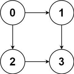
Input: graph = [[1,2],[3],[3],[]]
Output: [[0,1,3],[0,2,3]]
Explanation: There are two paths: 0 -> 1 -> 3 and 0 -> 2 -> 3.

Example 2:

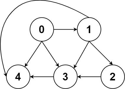
Input: graph = [[4,3,1],[3,2,4],[3],[4],[]]
Output: [[0,4],[0,3,4],[0,1,3,4],[0,1,2,3,4],[0,1,4]]

Code:

class Solution:
 def allPathsSourceTarget(self, graph: List[List[int]]) -> List[List[int]]:

 hash_map = {i:graph[i] for i in range(len(graph))}
 result, interm_res, current_node = [], [], 0
 self.retrieve_path(hash_map, result, interm_res, current_node)
 return result

 def retrieve_path(self, hash_map, result, interm_res, current_node):
 if current_node == len(hash_map.keys()) - 1:
 result.append(interm_res + [current_node])
 elif hash_map[current_node]:
 for i in hash_map[current_node]:
 self.retrieve_path(hash_map, result, interm_res+[current_node], i)

Explanation:

- allPathsSourceTarget Method:
 * Takes the graph which contains list of lists as input.
 * Step one will be mapping this directions to the nodes, 
 So created a dictionary to store nodes and directions information.
 * Initializing two lists - result to collect all the paths found and,
 interm_res to store intermediate path under construction and,
 current_node to track the current node.
 * Finally a call to retrieve_path method, which takes all the above
 variables as input.
- retrieve_path Method:
 * This method uses recursion to perform backtracking and find all the 
 possible paths.
 * For recursion we need a termination condition, and here if the current_node
 is equal to the last number in the list then it represents that path has 
 found, so it appends iterm_list with current_node and appends it to result.
 * if current_node has connections, as in,in the example -1, [0,1,2] has 
 connections but 3 doesn't have connections, if connections exist, 
 then code iterates through them to find possible paths
 * For each connection code performs a recursive call to the method by passing
 the updated parameters untill all the connections are explored.

3. N-Queens

The n-queens puzzle is the problem of placing n queens on an n x n chessboard such that no two queens attack each other.

Given an integer n, return the number of distinct solutions to the n-queens puzzle.

Example 1:

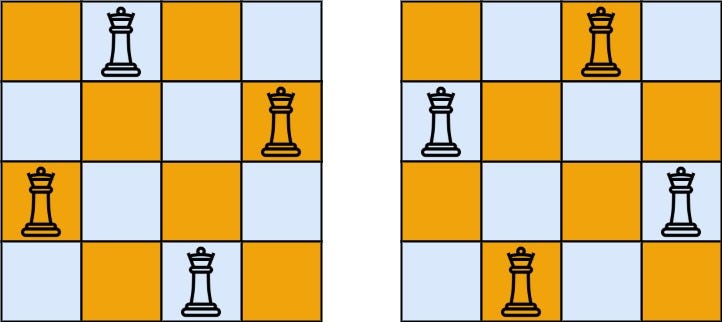
Input: n = 4
Output: 2
Explanation: There are two distinct solutions to the 4-queens puzzle as shown.

Example 2:

Input: n = 1
Output: 1

Code:

class Solution:
 def totalNQueens(self, n: int) -> int:
 def is_safe(board, current_queen, col):
 for i in range(current_queen):
 if board[i] == col or \
 board[i] - i == col - current_queen or \
 board[i] + i == col + current_queen:
 return False
 return True

 def solve(current_queen):
 if current_queen== n:
 nonlocal count
 count += 1
 return
 for col in range(n):
 if is_safe(board, current_queen, col):
 board[current_queen] = col
 solve(current_queen+ 1)
 
 board = [-1] * n
 count = 0
 solve(0)
 return count

Explanation:

* totalNQueens method is used to calculate N Queens where N represents number 
 of queens possible in N*N Chess Board.
* is_safe function checks whether it is safe to place a queen at a given 
 position on the chess board. It iterates through the straight portions and
 diagnols of queen and returns True if it is safe and viceversa.
* solve is reqcursive function which places all the queens on the chess board.
* if current_queen equals to n, it means all the queens are placed on the board
 so result is incremented by 1.
* Else it checks for each position in that row by making a recursive call and 
 tries to place the queen, if safe in a position goes to next queen in the 
 next row.
* Process continues till all the positions are successfully explored.

Optimization and Pruning in Backtracking

Although we covered basic examples, there are many ways to optimize backtracking, and instead of searching all the possible solutions, backtracking can also be used to find the best or feasible solution. Early Exit or Constraint-Specific Programming can be implemented to stop backtracking once a solution is found or certain constraints are met.

Techniques such as symmetry breaking, forward checking, and bounding can be used to eliminate unproductive states and reduce the number of states. Further Dynamic Programming Approaches such as Memoization or Tabulation can be implemented along with backtracking to optimize the process.

Backtracking pitfalls

While Backtracking is useful in many cases, there are a few common pitfalls to watch out for when working on Backtracking.

• Exponential Time Complexity: Due to multiple recursions, they can have exponential time complexity in the worst case, making it impractical for larger problems.
• Memory Consumption: Recursive Backtracking can consume a significant amount of memory due to the recursive call stack, which can lead to stack overflow or memoryBoundErrors.
• Optimization Balance: Over-optimization can lead to missed solutions, while under-optimization can slow down the algorithm, so finding the optimal optimization can be challenging.

There are cons, and don’t forget the pros, because that’s how the universe is structured.

if you want to explore more problems on backtracking, use this link, which contains around 100 problems.

Mail me if you get stuck at any point, Happy to Help. Happy Coding….

Join thousands of data leaders on the AI newsletter. Join over 80,000 subscribers and keep up to date with the latest developments in AI. From research to projects and ideas. If you are building an AI startup, an AI-related product, or a service, we invite you to consider becoming a sponsor.

Published via Towards AI