Random Forest for Image Classification Using OpenCV

By Stefania Cristina on January 30, 2024 in OpenCV 0

The Random Forest algorithm forms part of a family of ensemble machine learning algorithms and is a popular variation of bagged decision trees. It also comes implemented in the OpenCV library.

In this tutorial, you will learn how to apply OpenCV’s Random Forest algorithm for image classification, starting with a relatively easier banknote dataset and then testing the algorithm on OpenCV’s digits dataset.

After completing this tutorial, you will know:

Several of the most important characteristics of the Random Forest algorithm.
How to use the Random Forest algorithm for image classification in OpenCV.

Kick-start your project with my book Machine Learning in OpenCV. It provides self-study tutorials with working code.

Let’s get started.

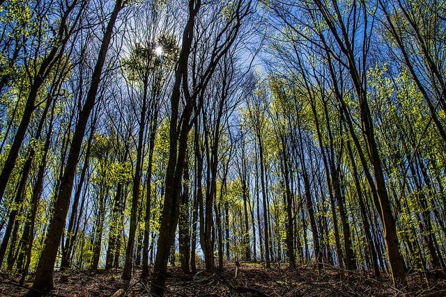
Random Forest for Image Classification Using OpenCV
Photo by Jeremy Bishop, some rights reserved.

Tutorial Overview

This tutorial is divided into two parts; they are:

Reminder of How Random Forests Work
Applying the Random Forest Algorithm to Image Classification
- Banknote Case Study
- Digits Case Study

Reminder of How Random Forests Work

The topic surrounding the Random Forest algorithm has already been explained well in these tutorials by Jason Brownlee [1, 2], but let’s first start with brushing up on some of the most important points:

Random Forest is a type of ensemble machine learning algorithm called bagging. It is a popular variation of bagged decision trees.

A decision tree is a branched model that consists of a hierarchy of decision nodes, where each decision node splits the data based on a decision rule. Training a decision tree involves a greedy selection of the best split points (i.e., points that divide the input space best) by minimizing a cost function.

The greedy approach through which decision trees construct their decision boundaries makes them susceptible to high variance. This means that small changes in the training dataset can lead to very different tree structures and, in turn, model predictions. If the decision tree is not pruned, it will also tend to capture noise and outliers in the training data. This sensitivity to the training data makes decision trees susceptible to overfitting.

Bagged decision trees address this susceptibility by combining the predictions from multiple decision trees, each trained on a bootstrap sample of the training dataset created by sampling the dataset with replacement. The limitation of this approach stems from the fact that the same greedy approach trains each tree, and some samples may be picked several times during training, making it very possible that the trees share similar (or the same) split points (hence, resulting in correlated trees).

The Random Forest algorithm tries to mitigate this correlation by training each tree on a random subset of the training data, created by randomly sampling the dataset without replacement. In this manner, the greedy algorithm can only consider a fixed subset of the data to create the split points that make up each tree, which forces the trees to be different.

In the case of a classification problem, every tree in the forest produces a prediction output, and the final class label is identified as the output that the majority of the trees have produced. In the case of regression, the final output is the average of the outputs produced by all the trees.

Applying the Random Forest Algorithm to Image Classification

Banknote Case Study

We’ll first use the banknote dataset used in this tutorial.

The banknote dataset is a relatively simple one that involves predicting a given banknote’s authenticity. The dataset contains 1,372 rows, with each row representing a feature vector comprising four different measures extracted from a banknote photograph, plus its corresponding class label (authentic or not).

The values in each feature vector correspond to the following:

Variance of Wavelet Transformed image (continuous)
Skewness of Wavelet Transformed image (continuous)
Kurtosis of Wavelet Transformed image (continuous)
Entropy of image (continuous)
Class label (integer)

The dataset may be downloaded from the UCI Machine Learning Repository.

Want to Get Started With Machine Learning with OpenCV?

Take my free email crash course now (with sample code).

Click to sign-up and also get a free PDF Ebook version of the course.

As in Jason’s tutorial, we shall load the dataset, convert its string numbers to floats, and partition it into training and testing sets:

# Function to load the dataset
def load_csv(filename):
    file = open(filename, "rt")
    lines = reader(file)
    dataset = list(lines)
    return dataset

# Function to convert a string column to float
def str_column_to_float(dataset, column):
    for row in dataset:
        row[column] = float32(row[column].strip())

# Load the dataset from text file
data = load_csv('Data/data_banknote_authentication.txt')

# Convert the dataset string numbers to float
for i in range(len(data[0])):
    str_column_to_float(data, i)

# Convert list to array
data = array(data)

# Separate the dataset samples from the ground truth
samples = data[:, :4]
target = data[:, -1, newaxis].astype(int32)

# Split the data into training and testing sets
x_train, x_test, y_train, y_test = ms.train_test_split(samples, target, test_size=0.2, random_state=10)

# Function to load the dataset

def load_csv(filename):

file = open(filename, "rt")

lines = reader(file)

dataset = list(lines)

return dataset

# Function to convert a string column to float

def str_column_to_float(dataset, column):

for row in dataset:

row[column] = float32(row[column].strip())

# Load the dataset from text file

data = load_csv('Data/data_banknote_authentication.txt')

# Convert the dataset string numbers to float

for i in range(len(data[0])):

str_column_to_float(data, i)

# Convert list to array

data = array(data)

# Separate the dataset samples from the ground truth

samples = data[:, :4]

target = data[:, -1, newaxis].astype(int32)

# Split the data into training and testing sets

x_train, x_test, y_train, y_test = ms.train_test_split(samples, target, test_size=0.2, random_state=10)

The OpenCV library implements the RTrees_create function in the ml module, which will allow us to create an empty decision tree:

# Create an empty decision tree
rtree = ml.RTrees_create()

1 2	# Create an empty decision tree rtree = ml.RTrees_create()

All the trees in the forest will be trained with the same parameter values, albeit on different subsets of the training dataset. The default parameter values can be customized, but let’s first work with the default implementation. We will return to customizing these parameter values shortly in the next section:

# Train the decision tree
rtree.train(x_train, ml.ROW_SAMPLE, y_train)

# Predict the target labels of the testing data
_, y_pred = rtree.predict(x_test)

# Compute and print the achieved accuracy
accuracy = (sum(y_pred.astype(int32) == y_test) / y_test.size) * 100
print('Accuracy:', accuracy[0], '%')

# Train the decision tree

rtree.train(x_train, ml.ROW_SAMPLE, y_train)

# Predict the target labels of the testing data

_, y_pred = rtree.predict(x_test)

# Compute and print the achieved accuracy

accuracy = (sum(y_pred.astype(int32) == y_test) / y_test.size) * 100

print('Accuracy:', accuracy[0], '%')

Accuracy: 96.72727272727273 %

1	Accuracy: 96.72727272727273 %

We have already obtained a high accuracy of around 96.73% using the default implementation of the Random Forest algorithm on the banknote dataset.

The complete code listing is as follows:

from csv import reader
from numpy import array, float32, int32, newaxis
from cv2 import ml
from sklearn import model_selection as ms

# Function to load the dataset
def load_csv(filename):
    file = open(filename, "rt")
    lines = reader(file)
    dataset = list(lines)
    return dataset

# Function to convert a string column to float
def str_column_to_float(dataset, column):
    for row in dataset:
        row[column] = float32(row[column].strip())


# Load the dataset from text file
data = load_csv('Data/data_banknote_authentication.txt')

# Convert the dataset string numbers to float
for i in range(len(data[0])):
    str_column_to_float(data, i)

# Convert list to array
data = array(data)

# Separate the dataset samples from the ground truth
samples = data[:, :4]
target = data[:, -1, newaxis].astype(int32)

# Split the data into training and testing sets
x_train, x_test, y_train, y_test = ms.train_test_split(samples, target, test_size=0.2, random_state=10)

# Create an empty decision tree
rtree = ml.RTrees_create()

# Train the decision tree
rtree.train(x_train, ml.ROW_SAMPLE, y_train)

# Predict the target labels of the testing data
_, y_pred = rtree.predict(x_test)

# Compute and print the achieved accuracy
accuracy = (sum(y_pred.astype(int32) == y_test) / y_test.size) * 100
print('Accuracy:', accuracy[0], '%')

from csv import reader

from numpy import array, float32, int32, newaxis

from cv2 import ml

from sklearn import model_selection as ms

# Function to load the dataset

def load_csv(filename):

file = open(filename, "rt")

lines = reader(file)

dataset = list(lines)

return dataset

# Function to convert a string column to float

def str_column_to_float(dataset, column):

for row in dataset:

row[column] = float32(row[column].strip())

# Load the dataset from text file

data = load_csv('Data/data_banknote_authentication.txt')

# Convert the dataset string numbers to float

for i in range(len(data[0])):

str_column_to_float(data, i)

# Convert list to array

data = array(data)

# Separate the dataset samples from the ground truth

samples = data[:, :4]

target = data[:, -1, newaxis].astype(int32)

# Split the data into training and testing sets

x_train, x_test, y_train, y_test = ms.train_test_split(samples, target, test_size=0.2, random_state=10)

# Create an empty decision tree

rtree = ml.RTrees_create()

# Train the decision tree

rtree.train(x_train, ml.ROW_SAMPLE, y_train)

# Predict the target labels of the testing data

_, y_pred = rtree.predict(x_test)

# Compute and print the achieved accuracy

accuracy = (sum(y_pred.astype(int32) == y_test) / y_test.size) * 100

print('Accuracy:', accuracy[0], '%')

Digits Case Study

Consider applying the Random Forest to images from OpenCV’s digits dataset.

The digits dataset is still relatively simple. However, the feature vectors we will extract from its images using the HOG method will have higher dimensionality (81 features) than those in the banknote dataset. For this reason, we can consider the digits dataset to be relatively more challenging to work with than the banknote dataset.

We will first investigate how the default implementation of the Random Forest algorithm copes with higher-dimensional data:

from digits_dataset import split_images, split_data
from feature_extraction import hog_descriptors
from numpy import array, float32
from cv2 import ml


# Load the digits image
img, sub_imgs = split_images('Images/digits.png', 20)

# Obtain training and testing datasets from the digits image
digits_train_imgs, digits_train_labels, digits_test_imgs, digits_test_labels = split_data(20, sub_imgs, 0.8)

# Convert the image data into HOG descriptors
digits_train_hog = hog_descriptors(digits_train_imgs)
digits_test_hog = hog_descriptors(digits_test_imgs)

# Create an empty decision tree
rtree_digits = ml.RTrees_create()

# Predict the target labels of the testing data
_, digits_test_pred = rtree_digits.predict(digits_test_hog)

# Compute and print the achieved accuracy
accuracy_digits = (sum(digits_test_pred.astype(int) == digits_test_labels) / digits_test_labels.size) * 100
print('Accuracy:', accuracy_digits[0], '%')

from digits_dataset import split_images, split_data

from feature_extraction import hog_descriptors

from numpy import array, float32

from cv2 import ml

# Load the digits image

img, sub_imgs = split_images('Images/digits.png', 20)

# Obtain training and testing datasets from the digits image

digits_train_imgs, digits_train_labels, digits_test_imgs, digits_test_labels = split_data(20, sub_imgs, 0.8)

# Convert the image data into HOG descriptors

digits_train_hog = hog_descriptors(digits_train_imgs)

digits_test_hog = hog_descriptors(digits_test_imgs)

# Create an empty decision tree

rtree_digits = ml.RTrees_create()

# Predict the target labels of the testing data

_, digits_test_pred = rtree_digits.predict(digits_test_hog)

# Compute and print the achieved accuracy

accuracy_digits = (sum(digits_test_pred.astype(int) == digits_test_labels) / digits_test_labels.size) * 100

print('Accuracy:', accuracy_digits[0], '%')

Accuracy: 81.0 %

1	Accuracy: 81.0 %

We find that the default implementation returns an accuracy of 81%.

This drop in accuracy from that achieved on the banknote dataset may indicate that the capacity of the default implementation of the model may not be enough to learn the complexity of the higher-dimensional data that we are now working with.

Let’s investigate whether we may obtain an improvement in the accuracy by changing:

The termination criteria of the training algorithm, which considers the number of trees in the forest, and the estimated performance of the model are measured by an Out-Of-Bag (OOB) error. The current termination criteria may be found by making use of the getTermCriteria method and set using the setTermCriteria method. When using the latter, the number of trees may be set through the TERM_CRITERIA_MAX_ITER parameter, whereas the desired accuracy may be specified using the TERM_CRITERIA_EPS parameter.

The maximum possible depth that each tree in the forest can attain. The current depth may be found using the getMaxDepth method, and set using the setMaxDepth method. The specified tree depth may not be reached if the above termination criteria are met first.

When tweaking the above parameters, remember that increasing the number of trees can increase the model’s capacity to capture more intricate detail in the training data; it will also increase the prediction time linearly and make the model more susceptible to overfitting. Hence, tweak the parameters judiciously.

If we add in the following lines following the creation of an empty decision tree, we may find the default values of the tree depth as well as the termination criteria:

print('Default tree depth:', rtree_digits.getMaxDepth())
print('Default termination criteria:', rtree_digits.getTermCriteria())

1 2	print('Default tree depth:', rtree_digits.getMaxDepth()) print('Default termination criteria:', rtree_digits.getTermCriteria())

Default tree depth: 5
Default termination criteria: (3, 50, 0.1)

1 2	Default tree depth: 5 Default termination criteria: (3, 50, 0.1)

In this manner, we can see that, by default, each tree in the forest has a depth (or number of levels) equal to 5, while the number of trees and desired accuracy are set to 50 and 0.1, respectively. The first value returned by the getTermCriteria method refers to the type of termination criteria under consideration, where a value of 3 specifies termination based on both TERM_CRITERIA_MAX_ITER and TERM_CRITERIA_EPS.

Let’s now try changing the values mentioned above to investigate their effect on the prediction accuracy. The code listing is as follows:

from digits_dataset import split_images, split_data
from feature_extraction import hog_descriptors
from numpy import array, float32
from cv2 import ml, TERM_CRITERIA_MAX_ITER, TERM_CRITERIA_EPS


# Load the digits image
img, sub_imgs = split_images('Images/digits.png', 20)

# Obtain training and testing datasets from the digits image
digits_train_imgs, digits_train_labels, digits_test_imgs, digits_test_labels = split_data(20, sub_imgs, 0.8)

# Convert the image data into HOG descriptors
digits_train_hog = hog_descriptors(digits_train_imgs)
digits_test_hog = hog_descriptors(digits_test_imgs)

# Create an empty decision tree
rtree_digits = ml.RTrees_create()

# Read the default parameter values
print('Default tree depth:', rtree_digits.getMaxDepth())
print('Default termination criteria:', rtree_digits.getTermCriteria())

# Change the default parameter values
rtree_digits.setMaxDepth(15)
rtree_digits.setTermCriteria((TERM_CRITERIA_MAX_ITER + TERM_CRITERIA_EPS, 100, 0.01))

# Train the decision tree
rtree_digits.train(digits_train_hog.astype(float32), ml.ROW_SAMPLE, digits_train_labels)

# Predict the target labels of the testing data
_, digits_test_pred = rtree_digits.predict(digits_test_hog)

# Compute and print the achieved accuracy
accuracy_digits = (sum(digits_test_pred.astype(int) == digits_test_labels) / digits_test_labels.size) * 100
print('Accuracy:', accuracy_digits[0], ‘%')

from digits_dataset import split_images, split_data

from feature_extraction import hog_descriptors

from numpy import array, float32

from cv2 import ml, TERM_CRITERIA_MAX_ITER, TERM_CRITERIA_EPS

# Load the digits image

img, sub_imgs = split_images('Images/digits.png', 20)

# Obtain training and testing datasets from the digits image

digits_train_imgs, digits_train_labels, digits_test_imgs, digits_test_labels = split_data(20, sub_imgs, 0.8)

# Convert the image data into HOG descriptors

digits_train_hog = hog_descriptors(digits_train_imgs)

digits_test_hog = hog_descriptors(digits_test_imgs)

# Create an empty decision tree

rtree_digits = ml.RTrees_create()

# Read the default parameter values

print('Default tree depth:', rtree_digits.getMaxDepth())

print('Default termination criteria:', rtree_digits.getTermCriteria())

# Change the default parameter values

rtree_digits.setMaxDepth(15)

rtree_digits.setTermCriteria((TERM_CRITERIA_MAX_ITER + TERM_CRITERIA_EPS, 100, 0.01))

# Train the decision tree

rtree_digits.train(digits_train_hog.astype(float32), ml.ROW_SAMPLE, digits_train_labels)

# Predict the target labels of the testing data

_, digits_test_pred = rtree_digits.predict(digits_test_hog)

# Compute and print the achieved accuracy

accuracy_digits = (sum(digits_test_pred.astype(int) == digits_test_labels) / digits_test_labels.size) * 100

print('Accuracy:', accuracy_digits[0], ‘%')

Accuracy: 94.1 %

1	Accuracy: 94.1 %

We may see that the newly set parameter values bump the prediction accuracy to 94.1%.

These parameter values are being set arbitrarily here to illustrate this example. Still, it is always advised to take a more systematic approach to tweaking the parameters of a model and investigating how each affects its performance.

Summary

In this tutorial, you learned how to apply OpenCV’s Random Forest algorithm for image classification, starting with a relatively easier banknote dataset and then testing the algorithm on OpenCV’s digits dataset.

Specifically, you learned:

Several of the most important characteristics of the Random Forest algorithm.
How to use the Random Forest algorithm for image classification in OpenCV.

Do you have any questions?

Ask your questions in the comments below, and I will do my best to answer.

Get Started on Machine Learning in OpenCV!

Learn how to use machine learning techniques in image processing projects

...using OpenCV in advanced ways and work beyond pixels

Discover how in my new Ebook:
Machine Learing in OpenCV

It provides self-study tutorials with all working code in Python to turn you from a novice to expert. It equips you with
logistic regression, random forest, SVM, k-means clustering, neural networks, and much more...all using the machine learning module in OpenCV

Kick-start your deep learning journey with hands-on exercises

See What's Inside

Navigation

Random Forest for Image Classification Using OpenCV

Tutorial Overview

Reminder of How Random Forests Work

Applying the Random Forest Algorithm to Image Classification

Banknote Case Study

Want to Get Started With Machine Learning with OpenCV?

Digits Case Study

Further Reading

Books

Websites

Summary

Get Started on Machine Learning in OpenCV!

Learn how to use machine learning techniques in image processing projects

Kick-start your deep learning journey with hands-on exercises

More On This Topic

No comments yet.

Leave a Reply Click here to cancel reply.