Cross-Validation Techniques for Machine Learning: A Guide to Improve Model Performance
Understand Different Techniques and How to Use Them for Better Model Evaluation

We develop machine-learning models from data. We want these models to be as precise as possible. But the usefulness of a model actually is determined by its performance on future data. Therefore, we must find a way to make the most of the available data useful for future data.
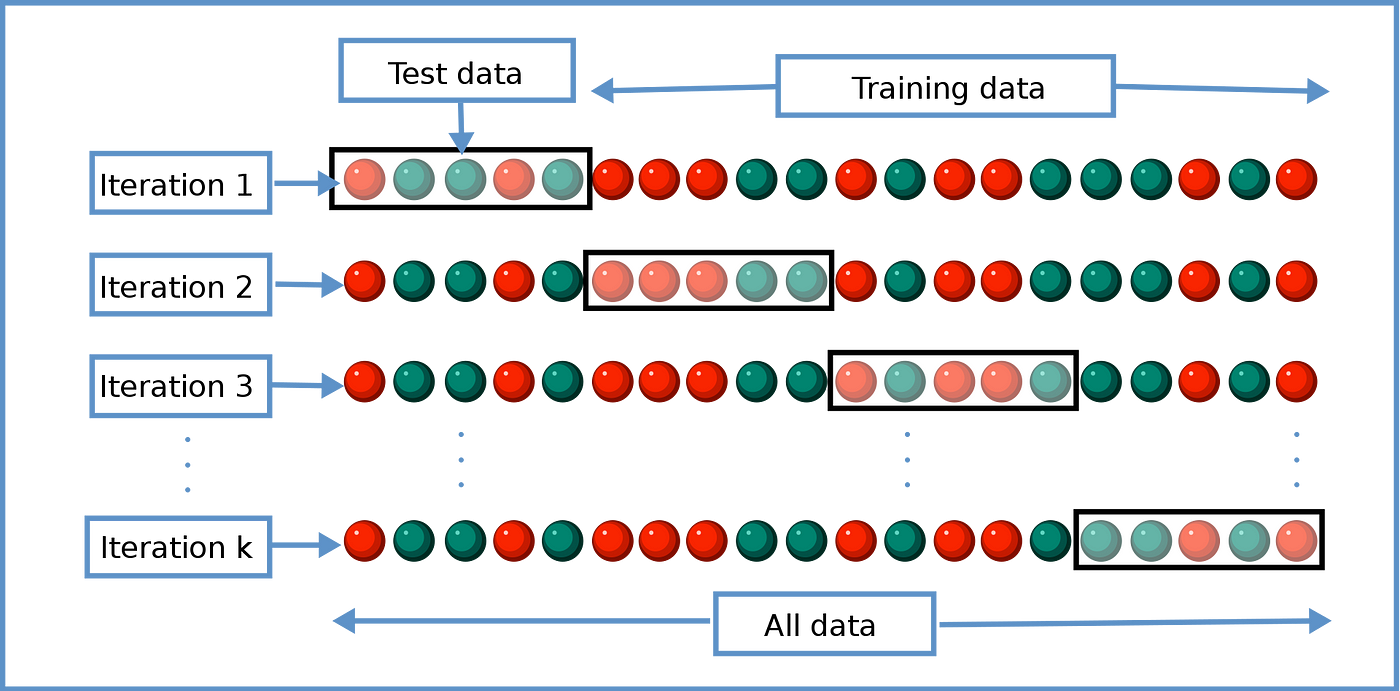
The available data are our training data. Since we do not have access to future data at the moment, we try to test the generalizability of the model we developed by separating some of the data we have from the training set and pretending that these are future data. We use some of the data for training and some for testing (we will not use test data for training). How we do this is the subject of the concept of cross-validation.

I will develop a model using the training data (blue) and apply it to my test data (red). I will check how well it was able to predict the future. With cross-validation methods, I will actually change this selection and division procedure dynamically and try to utilize all the data I have.
First, I randomly select 80% of my data for training and 20% for testing. Then I get another random 80% for training, and so on. By dividing the data into different subsets and training models on them, cross-validation allows the model to be trained on all of the available data, rather than a single train-test split.
Thus, I test the robustness and stability of my model. The model I provided with a single split was tested on only one test dataset. Maybe there were some situations in the split that I was not aware of. The inherent distributions of the features could not be fully reflected by the subsets. In this case, even if my result is good, generalization is actually insufficient and there is an overfitting situation (we can also call it a self-fulfilling prophecy). We should find the best model that performs well on each split.
Cross-validation is not actually (just) a validation process. It is more of a fine-tuning process. Our goal is not just to evaluate the performance of the model on unseen data but also to optimize the model’s performance by selecting the best model and tuning its hyperparameters. We train multiple models on different subsets and select the model with the best performance in the end.
There are several methods for performing cross-validation:
- K-Fold
- Leave-one-out
- Stratified K-Fold
- Monte Carlo cross-validation
- Bootstrapping
In each, we split the data into new train and test subsets. Then, we evaluate the models that we build. We take the average of all measures to get the actual performance metric.
Before diving deep into these methods, let’s first eliminate the simplest (one-way, one-time) split which is generally called the Hold Out method.
Hold Out Method
First, let’s load The Boston Housing Dataset from sklearn.
import pandas as pd
from sklearn.datasets import load_boston
boston = load_boston()
df = pd.DataFrame(data=boston.data, columns=boston.feature_names)
df["Target"] = boston.target
df.head()
print(df.shape) #(506, 14)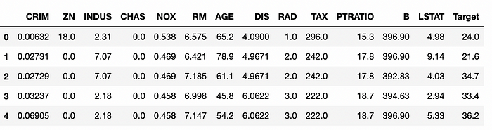
Let’s split the data. We are using train_test_split from sklearn.
X = boston.data
y = boston.target
from sklearn.model_selection import train_test_split
X_train, X_test, y_train, y_test = train_test_split(X, y, test_size=0.2, random_state=42)
print(X_train.shape) #(404, 13)
print(X_test.shape) #(102, 13)
The parameters that the train_test_split accepts:
test_size: It controls the proportion of the data that will be used for the test set. 0.2 means that 20% of the data will be used for testing. If we pass an integer value, then that represents the number of samples to use for the test set.train_size: Similar totest_sizebut it's used to set the size of the training set.random_state:random seed.shuffle: shuffle dataset before the split?stratify: is used to stratify the split, which ensures that the proportion of samples for each class is the same in both the train and test sets. This is important when working with imbalanced datasets.
Let’s run an XGBoost estimator to predict root mean square error.
import xgboost as xgb
import numpy as np
from sklearn.metrics import mean_squared_error
estimator = xgb.XGBRegressor(objective ='reg:squarederror', seed = 10)
estimator.fit(X_train, y_train)

# Predict the model
y_pred = estimator.predict(X_test)

# RMSE Evaluation
rmse = np.sqrt(mean_squared_error(y_test, y_pred))
print("RMSE: % f" %(rmse))
#RMSE:  2.561353
This method is quick and simple, even too simple. Many topics are out of scope. The observations we reserved for the test could not participate in the training process in any way.
OK, we have developed a simple machine-learning model. Now let’s introduce other (harder-better-stronger) cross-validation methods.
K-Fold
We divide our data into k number of sections. We use one section for testing and the rest for training.
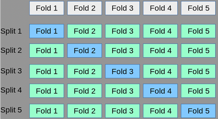
We have k (5) different models. The final performance measure will be the average of k models.
The standard deviation of the results of different iterations is as important as the average. Let’s say that one model has a good result, while the other has a very bad result. This shows us that there are some errors in the split operation.
from sklearn.model_selection import KFold
KFold has three parameters:
n_splits: k, number of folds.
Normally, people take k as 5 to 10. As the k value increases, there will be more iterations, so the computational cost will increase. So, if you have limited resources, use smaller k.
We should also consider the size of the dataset. A larger dataset (we can say that a dataset with at least 10,000 observations is large?) can tolerate a larger value of k. Conversely, we should select a smaller k value for small datasets (a dataset with 100 observations is small).
If your data is highly variable (high variance), it is better to use smaller k values to be able to represent this variance in each fold. In the opposite direction, if your data is more homogeneous, then you can switch to higher k values.
random_state: seedshuffle: Do you want to shuffle the dataset before the split?
from sklearn.model_selection import KFold
kf = KFold(n_splits=5)

print(kf)
#KFold(n_splits=5, random_state=None, shuffle=False)

#Generate indices to split data into training and test set.
fold_generator = kf.split(X)
print(fold_generator)
#<generator object _BaseKFold.split at 0x7f96e85e2dd0>

for i, (train_index, test_index) in enumerate(fold_generator):
    print(f"Fold {i}:")
    print(f"  Train: index={train_index}")
    print(f"  Test:  index={test_index}")

"""
Fold 0:
  Train: index=[102 103 104 105 106.....
  Test:  index=[  0   1   2   3   4   5  ....
Fold 1:
  Train: index=[  0   1   2   3   4   5   6  ..
....
"""
Let’s visualize the folds.
import matplotlib.pyplot as plt

fig = plt.figure(figsize = (12, 5))
colors = ["orange","red","blue","gray","black"]
counter = 0
for i, (train_index, test_index) in enumerate(kf.split(X)):
    plt.scatter(train_index,np.full_like(train_index, counter+1), c =colors[i])
    plt.scatter(test_index, np.full_like(test_index, counter), c =colors[i])
    counter += 2.5
plt.show()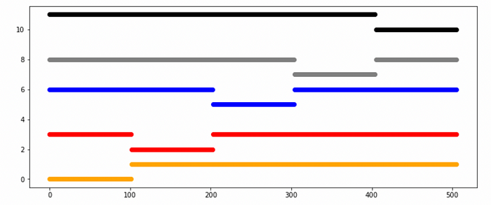
Let’s find the score of each model trained by a different fold.
import xgboost as xgb
estimator = xgb.XGBRegressor(seed=10)

scores = []
for train_index, test_index in kf.split(X):
    X_train, X_test = X[train_index], X[test_index]
    y_train, y_test = y[train_index], y[test_index]
    estimator.fit(X_train, y_train)
    scores.append(estimator.score(X_test, y_test)) #returns r2

# scores
print(scores) #[0.7343818374985939, 0.8490298604014259, 0.8257969178459365, 0.5237461839046007, 0.29743000915088447]
print(np.mean(scores)) #0.6460769617602883
We can also use the cross_val_score method to handle the same thing in one line of code.
from sklearn.model_selection import cross_val_score
result = cross_val_score(estimator , X, y, cv = kf, scoring="r2")
print(result)
#[0.73438184 0.84902986 0.82579692 0.52374618 0.29743001]
We can pass our KFold object to GridSearchCV to tune hyperparameters.
from sklearn.model_selection import GridSearchCV

model = XGBRegressor()

# hyperparameter grid
param_grid = {'max_depth': [3, 5, 7], 'learning_rate': [0.1, 0.2, 0.3]}

grid_search = GridSearchCV(model, param_grid, cv=kf)
grid_search.fit(X, y)
print(grid_search.best_params_)
#{'learning_rate': 0.1, 'max_depth': 3}
Let me share a little tip here: don’t buy every result that GridSearchCV gives. Be sure to review the CV results. The standard deviation of these results is as important as the mean. Rather than choosing the model with the worst standard deviation but the best average, a more robust model with a low deviation can be chosen by giving up the average.
import pandas as pd
df = pd.DataFrame(grid_search.cv_results_)
print(df)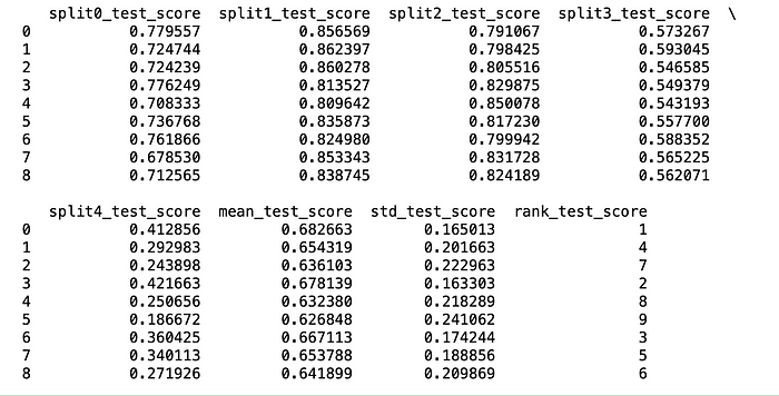
With KFold, we used all the observations in the training process. However, while doing this, we ignored the distribution of the features, just like in the hold-out method.
Stratified K-Fold
We divide the data in such a way that each subset contains certain groups with the same percentage. We use this method if we are dealing with unbalanced datasets.
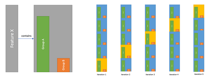
For example, feature X contains 2 class groups. While performing the partitioning process, we pay attention to the ratio between these 2 groups and we split in such a way that this ratio is the same among folds. That is the difference with the normal K-Fold method, paying attention to these distributions when making the split.
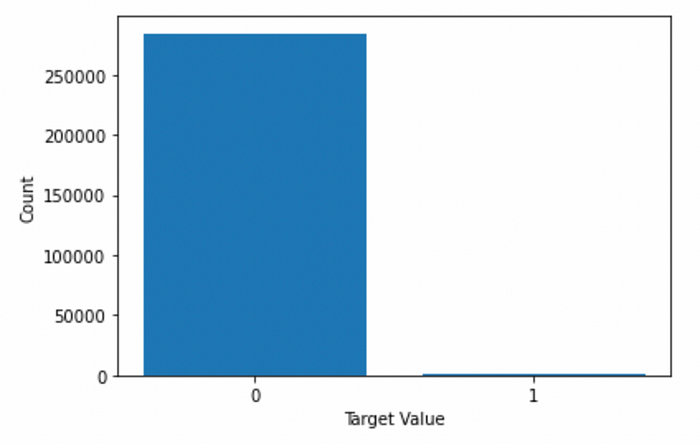
Here, I will use the credit card fraud detection dataset as a more appropriate example. This dataset's target “Class” feature has a highly unbalanced distribution.
import pandas as pd
data = pd.read_csv("creditcard.csv")
data.head()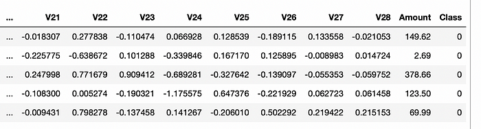
import matplotlib.pyplot as plt
data.dropna(inplace=True)
counts = data["Class"].value_counts()
plt.bar(counts.index, counts.values)
plt.xlabel("Target Value")
plt.ylabel("Count")
plt.xticks([0, 1])
plt.show()
print(counts)
"""
0    284315
1       492
Name: Class, dtype: int64
"""
import numpy as np
import xgboost as xgb
from sklearn.model_selection import StratifiedKFold

X = data.drop(['Class'], axis=1)
y = data['Class']

skf = StratifiedKFold(n_splits=5)
estimator = xgb.XGBClassifier(seed=10)

for train_index, test_index in skf.split(X, y):
    X_train, X_test = X.iloc[train_index], X.iloc[test_index]
    y_train, y_test = y.iloc[train_index], y.iloc[test_index]
    estimator.fit(X_train, y_train)
    y_pred = estimator.predict(X_test)
    print(f"Fold Distribution of Train: {np.bincount(y_train)} - Test: {np.bincount(y_test)}")

"""
Fold Distribution of Train: [227452    393] - Test: [56863    99]
Fold Distribution of Train: [227452    393] - Test: [56863    99]
Fold Distribution of Train: [227452    394] - Test: [56863    98]
Fold Distribution of Train: [227452    394] - Test: [56863    98]
Fold Distribution of Train: [227452    394] - Test: [56863    98]
"""
import numpy as np
import xgboost as xgb
from sklearn.model_selection import StratifiedKFold
from sklearn.metrics import classification_report
X = data.drop(['Class'], axis=1)
y = data['Class']
skf = StratifiedKFold(n_splits=5)
estimator = xgb.XGBClassifier(seed=10)
for train_index, test_index in skf.split(X, y):
X_train, X_test = X.iloc[train_index], X.iloc[test_index]
y_train, y_test = y.iloc[train_index], y.iloc[test_index]
estimator.fit(X_train, y_train)
y_pred = estimator.predict(X_test)
print(classification_report(y_test, y_pred))
"""
precision recall f1-score support
0 1.00 0.97 0.99 56863
1 0.06 0.96 0.11 99
accuracy 0.97 56962
macro avg 0.53 0.97 0.55 56962
weighted avg 1.00 0.97 0.98 56962
precision recall f1-score support
0 1.00 1.00 1.00 56863
1 0.96 0.76 0.85 99
accuracy 1.00 56962
macro avg 0.98 0.88 0.92 56962
weighted avg 1.00 1.00 1.00 56962
precision recall f1-score support
.
.
.
"""from sklearn.model_selection import cross_val_score
estimator = xgb.XGBClassifier(seed=10)
result = cross_val_score(estimator , X, y, cv = skf, scoring="accuracy")
print(result)
#[0.97180577 0.999526 0.99899932 0.99963133 0.99943821]We can apply StratifiedKFold with GridSearchCV
from sklearn.model_selection import GridSearchCV
estimator = xgb.XGBClassifier(seed=10)
skf = StratifiedKFold(n_splits=5)
# hyperparameter grid
param_grid = {'max_depth': [3, 5], 'learning_rate': [0.1, 0.2]}
grid_search = GridSearchCV(estimator, param_grid, cv=skf)
grid_search.fit(X, y)
print(grid_search.best_params_)
#{'learning_rate': 0.2, 'max_depth': 5}

import pandas as pd
df = pd.DataFrame(grid_search.cv_results_)
print(df)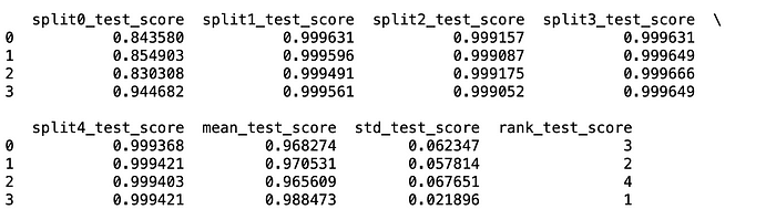
Leave One Out
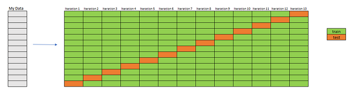
We use only one data point for testing and use the rest of the entire dataset (N-1) for training. Actually, k (k from K-fold) is equal to N here.
Imagine that I have a dataset containing 13 rows. So, I will train 13 models. I will have performance measurements for 13 models. We can take the average as the final measurement.
The biggest drawback of this method (which we can notice immediately) is that if your dataset is large enough, your computational cost will be very high.
We can use this in case our dataset is relatively small.
#Let's go back to the Boston dataset
from sklearn.model_selection import LeaveOneOut
loo = LeaveOneOut()
fold_generator = loo.split(X)
for i, (train_index, test_index) in enumerate(fold_generator):
print(f"Fold {i}:")
print(f" Train: index={len(train_index)}")
print(f" Test: index={len(test_index)}")
"""
Fold 0:
Train: index=505
Test: index=1
Fold 1:
Train: index=505
Test: index=1
Fold 2:
Train: index=505
Test: index=1
Fold 3:
Train: index=505
Test: index=1
.
.
.
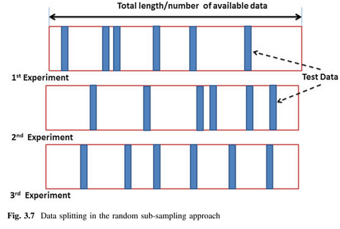
"""Monte Carlo Cross Validation
It is also called Repeated Random Sub-sampling Validation. Just like KFold, we split our data into folds again. However, folds are not predefined. The data is randomly split into training and test sets for each iteration.
We can use ShuffleSplit from sklearn.
from sklearn.model_selection import ShuffleSplit
shuffle=ShuffleSplit(test_size=0.2,train_size=0.8,n_splits=5)
for i, (train_index, test_index) in enumerate(shuffle.split(X)):
    print(f"Fold {i}:")
    print(f"  Train: index={train_index}")
    print(f"  Test:  index={test_index}")

"""
Fold 0:
  Train: index=[154 367 362 336  86 442 282  ...
  Test:  index=[251  14 238 107 484 ...
Fold 1:
  Train: index=[250 300  11 104 437  80 ...
  Test:  index=[261 232 382 376  18 468  ...
.
.
.
"""
Note that some observations may never be selected when using MCCV. This will potentially introduce bias to the system.
Bootstrapping
Bootstrapping is another technique to evaluate models. We estimate the distribution of a statistic by repeatedly sampling the data with replacement. It can be used as an alternative to cross-validation when the data set is small or when it is not feasible to split the data into separate training and testing sets. Bootstrapping can also be used to estimate the uncertainty of a model’s performance by generating multiple samples of the data and training the model on each sample.
In short, we randomly generate new datasets from the data we have.
In Bootstrapping, duplication is possible. So, let’s say you selected the first row r1, while choosing a second row it is possible to select row r1 again. In other words, the datasets you generate will likely have repetitive and missing rows compared to the original.
We can use resample method of sklearn to create a new random dataset.
import numpy as np
from sklearn.utils import resample

# the number of bootstrap samples to draw
n_iter = 100

# train test split percentage
percentage = 0.8
for i in range(n_iter):
    X_train, y_train = resample(X, y, replace=True, n_samples=int(X.shape[0]*percentage))
    X_test, y_test = resample(X, y, replace=True, n_samples=int(X.shape[0]*(1-percentage)))
    print(f"Shapes: X_train: {X_train.shape} y_train: {y_train.shape} X_test: {X_test.shape} y_test: {y_test.shape}")

"""
Shapes: X_train: (404, 13) y_train: (404,) X_test: (101, 13) y_test: (101,)
Shapes: X_train: (404, 13) y_train: (404,) X_test: (101, 13) y_test: (101,)
Shapes: X_train: (404, 13) y_train: (404,) X_test: (101, 13) y_test: (101,)
Shapes: X_train: (404, 13) y_train: (404,) X_test: (101, 13) y_test: (101,)
Shapes: X_train: (404, 13) y_train: (404,) X_test: (101, 13) y_test: (101,)
Shapes: X_train: (404, 13) y_train: (404,) X_test: (101, 13) y_test: (101,)
"""
CV is a good choice if our goal is to get a robust estimate of the model’s performance on unseen data and the size of the dataset is large enough to support it. On the other hand, we can use bootstrapping if the dataset is small and we aim to find out the uncertainty of the model’s performance.
Conclusion
We use cross-validation to evaluate and tune machine learning models by simply dividing the data into subsets, and to train and test a model with different subsets. It helps us to prevent overfitting, and find the best hyperparameter set for a model.
Read More
Sources
https://en.wikipedia.org/wiki/Cross-validation_(statistics)
https://scikit-learn.org/stable/modules/cross_validation.html
https://www.section.io/engineering-education/how-to-implement-k-fold-cross-validation/
https://stats.stackexchange.com/questions/51416/k-fold-vs-monte-carlo-cross-validation