The K-Nearest Neighbors Algorithm Math Foundations: Hyperplanes, Voronoi Diagrams and Spacial Metrics.
Throughout this article we’ll dissect the math behind one of the most famous, simple and old algorithms in all statistics and machine learning history: the KNN.
1. A little historical context
The year was 1951. Korean war blasting off all the nuclear fears of the Cold War Era. F-86 sabre jets and MiG-15s burning in the eastern sky. The USAF had just gained its independence from the army and, among explosions and cloudy political acts, two sharp-minded statisticians were developing some very cool work in the safety of the Twentieth Air Force intel office.
Evelyn Fix and Joseph Hodges wrote a technical report that brought the KNN algorithm discussed here to life.
2. The problem
Suppose you work at an aircraft factory. However, you are a robot that walks around the factory counting the number of planes produced and identifying their types. It is your duty to correctly classify them into their respective classes: military and small civil/commercial aircraft. To do so, you must recognize patterns by performing measurements.

You check, let’s say, two things on the planes you see: length and weight. By doing this work so many times, your robot brain learned how to get the measurements from its sensors and compare them to a library of previous knowledge to correctly classify the aircraft.

Every time you see a new plane coming out of the production line, you take its length and weight and, based on that info, you assign its type. In your 9-to-5, there are many lightweight jets like Phenom 300 and fighter jets like SU-57.

2.1 Intuition or what a model sees
Based on length and weight, your brain always visualizes the aircraft as in the chart below.
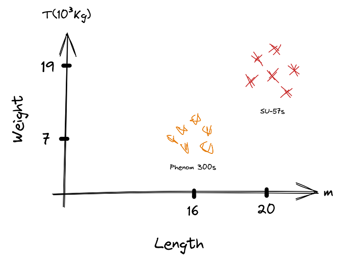
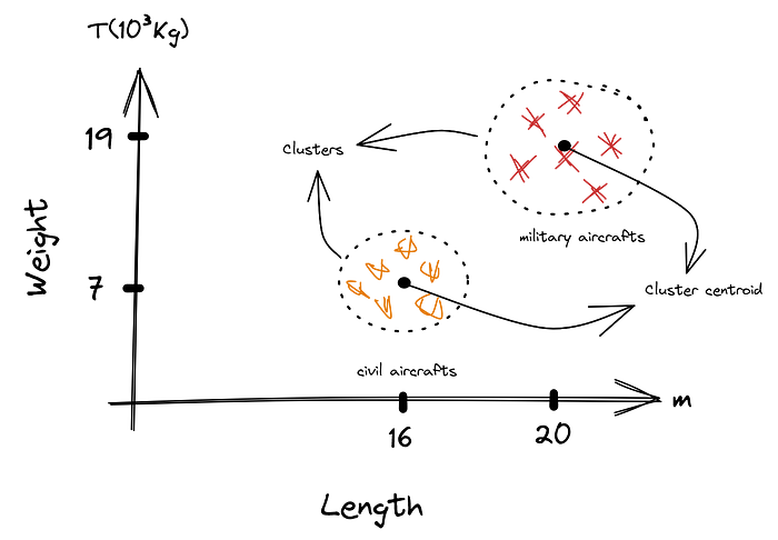
Phenoms and 57s are both clustered around their respective centroids.
2.3 K-Nearest Neighbors
Suppose that a new aircraft is being made. It is around 18 meters long and has about 9 tons. To classify a new aircraft, your brain would do the following
- Take a measure
- Graph it on the chart
- Check the distance from the new point to the nearby others already in the clusters
- Assign the class to the observed point as the same as the nearest clustered points
This is the K-NN algorithm. The ‘K’ depends on how many nearest points you are looking at. If K = 3, the chart would be
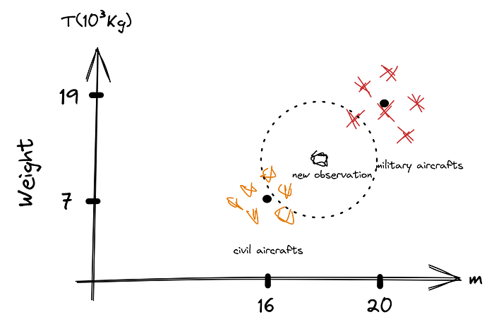
And the observed point would be classified as a civil aircraft.
2.4 Model Limitations and Wrong Classifications
It’s all right ‘till now. Whenever an airplane is about 16 meters long and 7 tons in weight, you classify it as a civil aircraft. Otherwise, it is certainly a military aircraft. These numbers — 16 m,7 T and 20 m,19 T — are the only ones you know for airplane classification. Whenever a measure approaches a cluster, you classify it as belonging to that cluster.
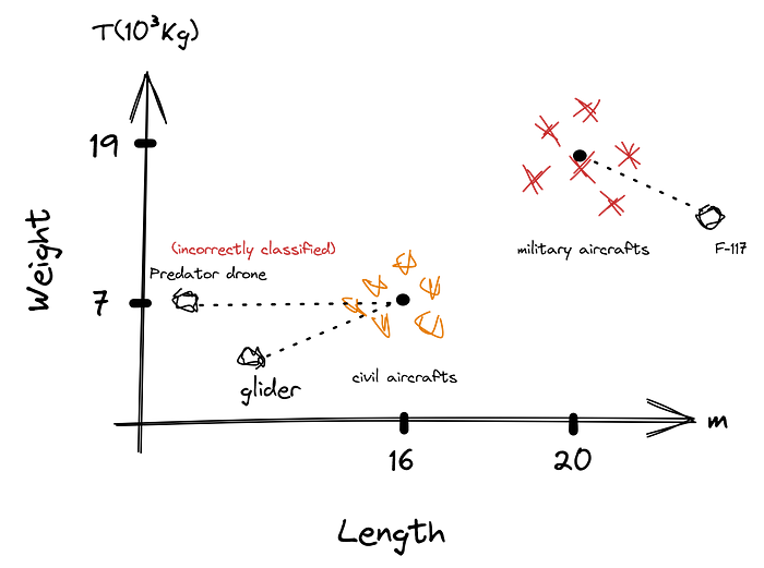
With this model, if you measure a glider, with half a ton of weight, or an F-117 Nighthawk, 20.1 meters long, it would all be correctly classified, based on distance from the point to the cluster’s centroid.
This model isn’t perfect, of course. A predator drone would be incorrectly classified as a civil aircraft, for example. To solve this problem, more dimensions would be needed on that chart — measures not only of weight and length, but also on wingspan, of crew and passengers and other relevant quantities. Also, would be suitable to create other clusters for civil and military drones, for example.
Enough with flying things.
3. The Math
Although it’s a simple problem, the inner machinations of picking the closest points are driven by some very interesting — and simple — math. In this session, we’ll look at three things: the Hyperplane Separation Theorem, the Voronoi regions and how to measure distances. At implementation time, the only thing really needed to know is how to measure distance. Feel free to skip the initial curious topics.
Disclaimer: our concern is with concepts and intuition. Mathematical rigor won’t be of importance here. Be advised.
3.1 Hyperplane Separation Theorem
Hyperplanes are extensions of normal planes. A normal plane exists in three-dimensional space and has two dimensions. A hyperplane is a mathematical object that exists in n-dimensional space and has a dimension of n-1.
Our statistical observations contain several dimensions.

Now suppose you have two non-empty sets that do not intersect with each other and are in a rounded shape with n dimensions in n-dimensional space. This is enough to affirm
There is a hyperplane that separates both sets and constitutes a barrier
between the elements of the sets. Observations on the left side of the
hyperplane belong to one class, and observations on the right side of
the hyperplane belong to another class.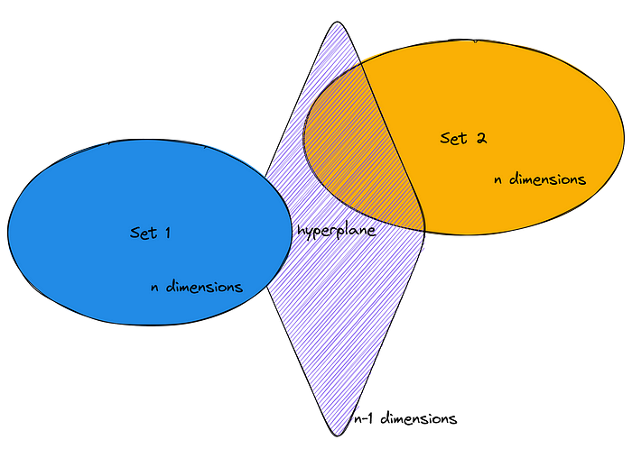
Check diagram 2 clusters.
These hyperplanes — also called hypersurfaces — are the decision boundaries of a KNN algorithm.
The intersection of several planes partitions the space into several Voronoi regions.
3.2 Voronoi Diagrams
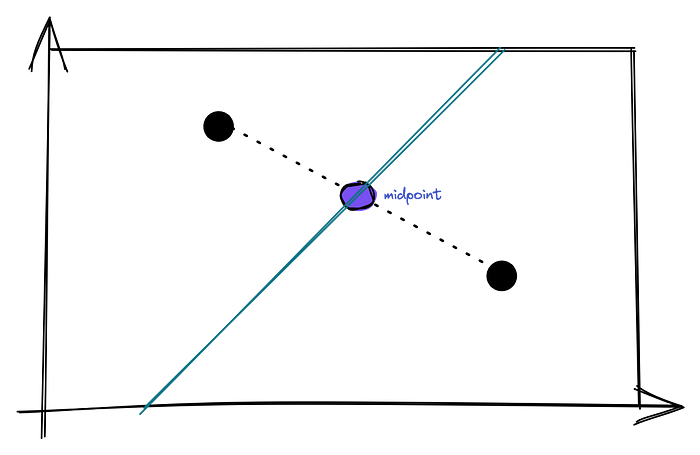
If our dataset is made up of various clusters and we have a really big dataset with a lot of labeled observations, we can partition the entire space into Voronoi regions. First, let’s tesselate a space with two clusters:

To tesselate or partition this space into the Voronoi regions, we’ll identify the midpoint of the line connecting the two points and graph another line orthogonal to the previous one:
And this can be done for any number of clusters or points:
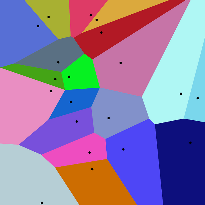
Where each region is a different class and a new observation that goes inside a region is labeled as of that class.
3.3 Measuring Distance
Distance is the amount of space between two points. These points will be our observations —the length of an aircraft — and the euclidean geometry allows us to measure the distance in two ways.
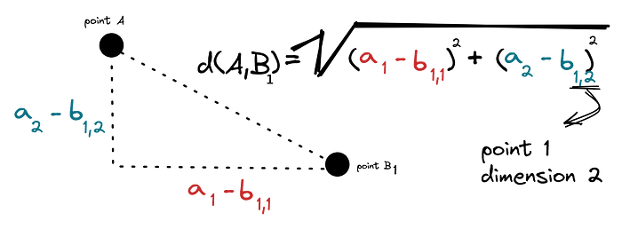
The Euclidean distance is the most well-known method for calculating distance. Let us imagine three points A, B and C with coordinates as depicted in the chart below.
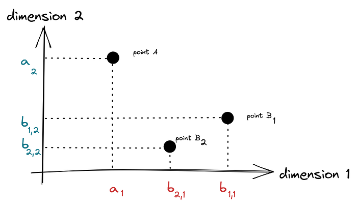
We measure the distance d(A,B) from A to B through the Pythagorean theorem:
Same goes for distance from A to C, d(A,C). We’re interested in the sum of the distances, d(A,B) + d(A,C):

Suppose now that there are M different points Bᵢ with N different dimensions each. We want the sum of the distances from A to all Bᵢ’s.


When dimensionality gets too big (big N), you can use the Manhattan distance:

The only difference between the Manhattan distance and euclidean distance is the squared sum argument and the square root. The Minkowski distance generalizes this difference in a simple expression:

And please note that the p argument is the one used in the Scikit-Learn library.
Conclusion
The content covered by this article is conceptual in nature and its objective is to formulate heuristics to develop a better understanding in implementation.
The next article will implement the KNN algorithm in Python using the Scikit-Learn library.
Thanks.
Do you identify as Latinx and are working in artificial intelligence or know someone who is Latinx and is working in artificial intelligence?
- Get listed on our directory and become a member of our member’s forum: https://forum.latinxinai.org/
- Become a writer for the LatinX in AI Publication by emailing us at publication@latinxinai.org
- Learn more on our website: http://www.latinxinai.org/
Don’t forget to hit the 👏 below to help support our community — it means a lot!
Thank you :)

